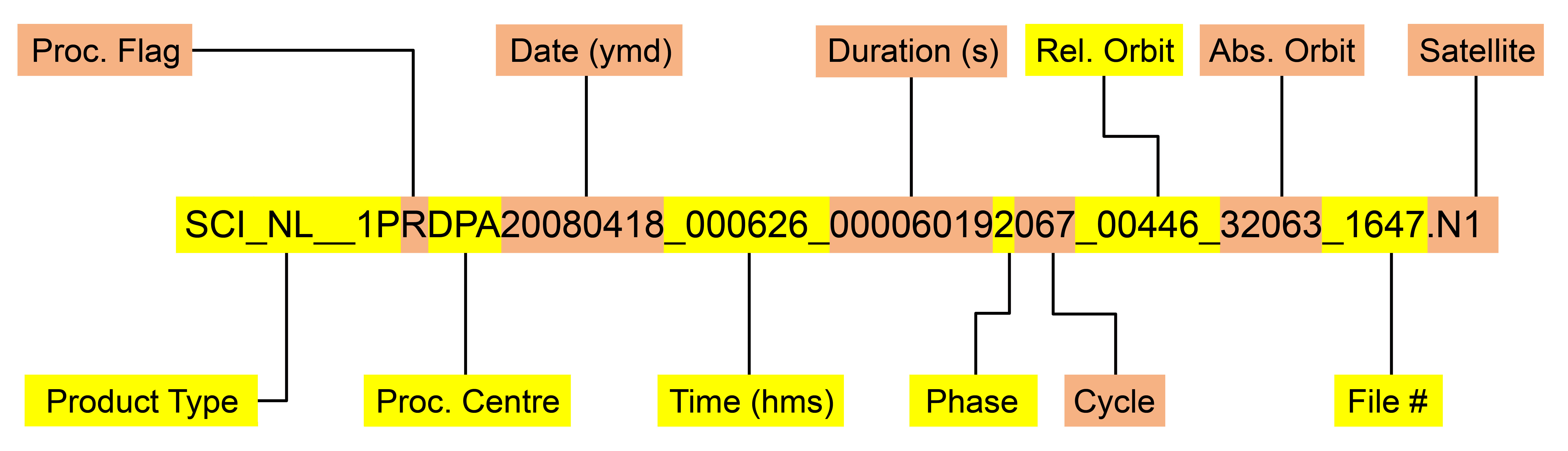
| Fig. 8-1 |
An example for a SCIAMACHY level 1b product filename illustrating the individual filename fields.
(Courtesy: DLR-IMF)
|
|
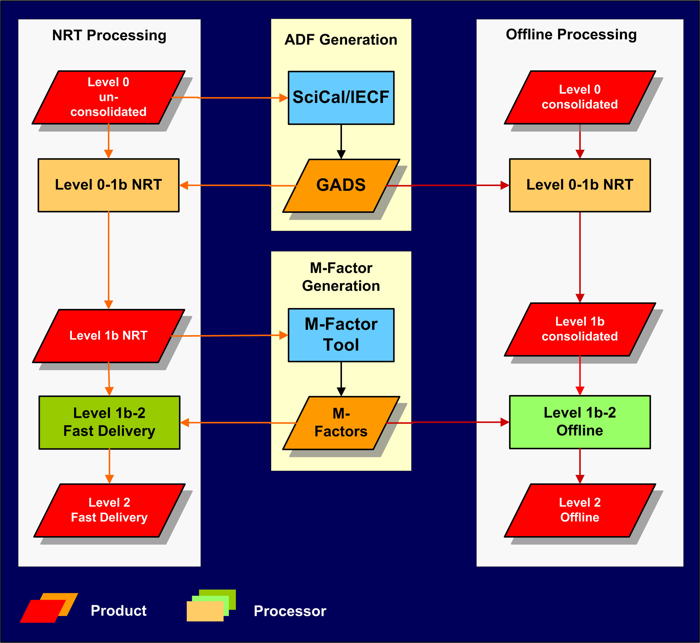
| Fig. 8-2 |
General processing flow in NRT/FD (left) and OL (right).
Both chains receive the calibration information from the same auxiliary flow.
(Courtesy: DLR-IMF)
|
|
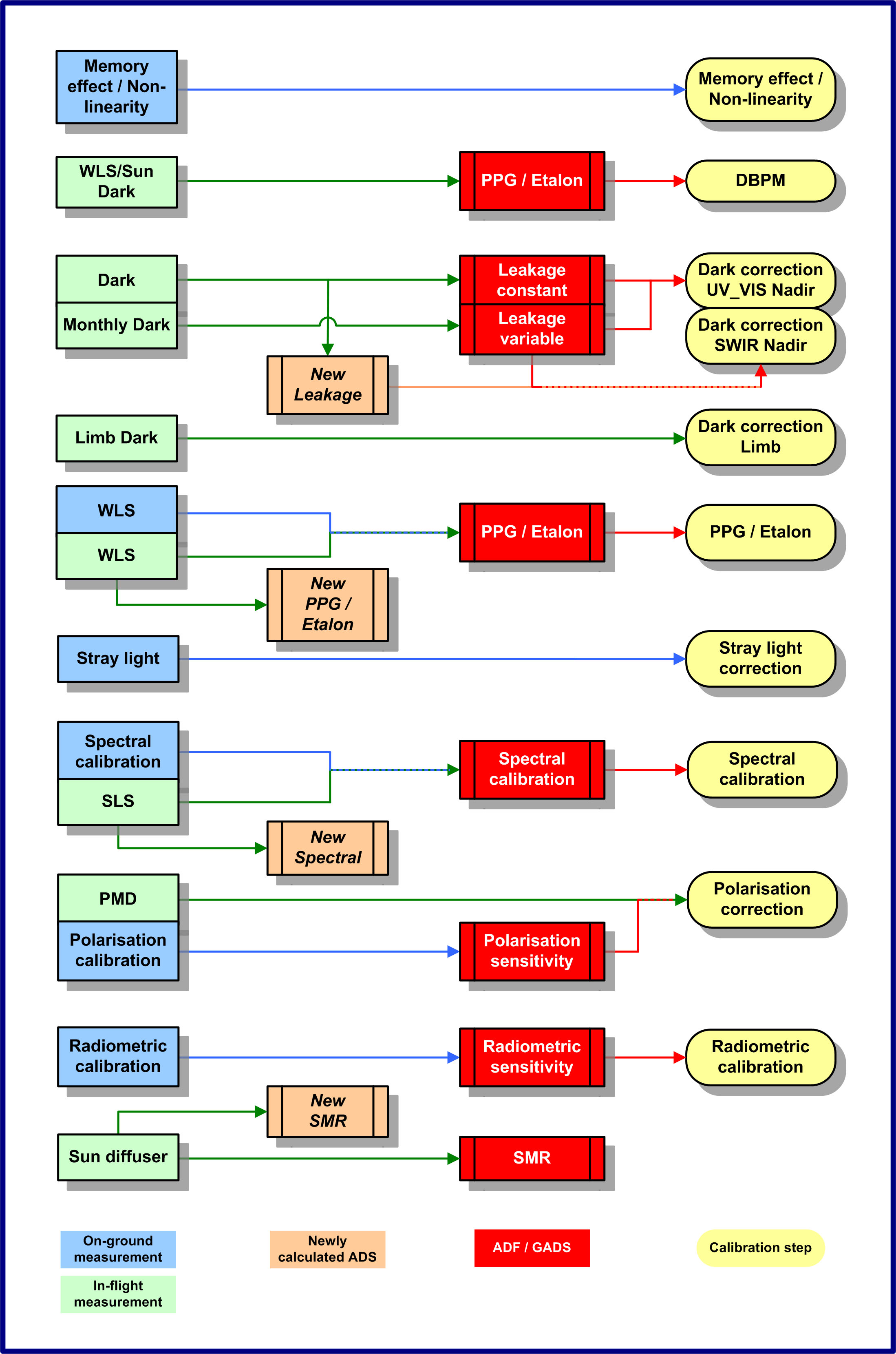
| Fig. 8-3 |
Relations between calibration measurements (blue: on-ground, green: in-flight), ADF/GADS (red),
newly calculated ADS (orange) and calibration steps (yellow). The calibration information is stored
either directly in the newly calculated ADS of the level 1b file or written into an ADF and subsequently
copied into the GADS of the level 1b file. Some calibration parameters, e.g. the stray light fractions, are
contained in the measurement datasets of the level 1b file. Except for the NEW LEAKAGE ADS, the newly calculated
ADS are not used in the standard calibration. (Courtesy: DLR-IMF)
|
|
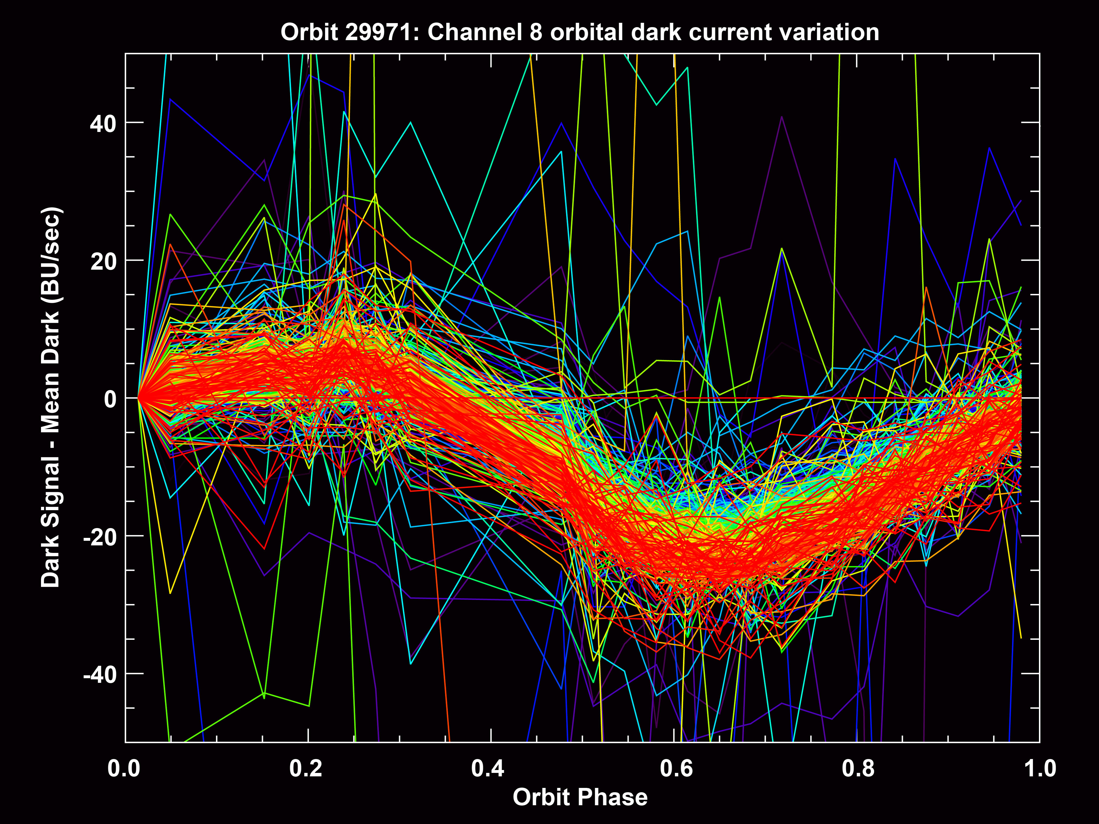
| Fig. 8-4 |
Orbital variation of the thermally induced dark signal for each pixel in channel 8. Orbit phase = 0
corresponds to eclipse entry. The Mean Dark is the dark signal per pixel averaged over a complete dark
current state close to phase 0. It permits to normalise the orbital variation at phase 0. (Courtesy: DLR-IMF)
|
|
| Fig. 8-5 |
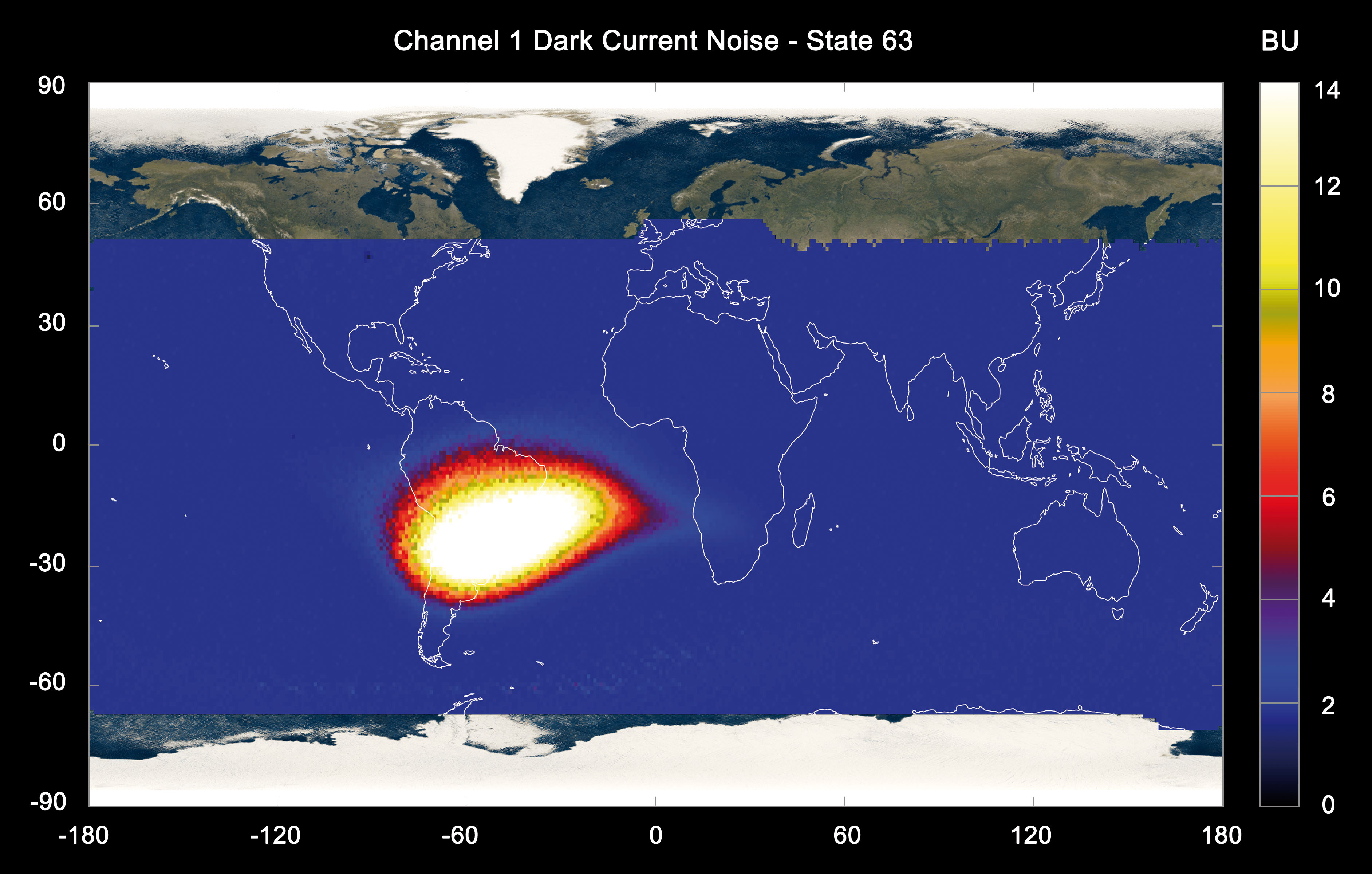
The SAA as derived from SCIAMACHY dark current measurements. (Courtesy: SRON)
|
 |
| Fig. 8-6 |
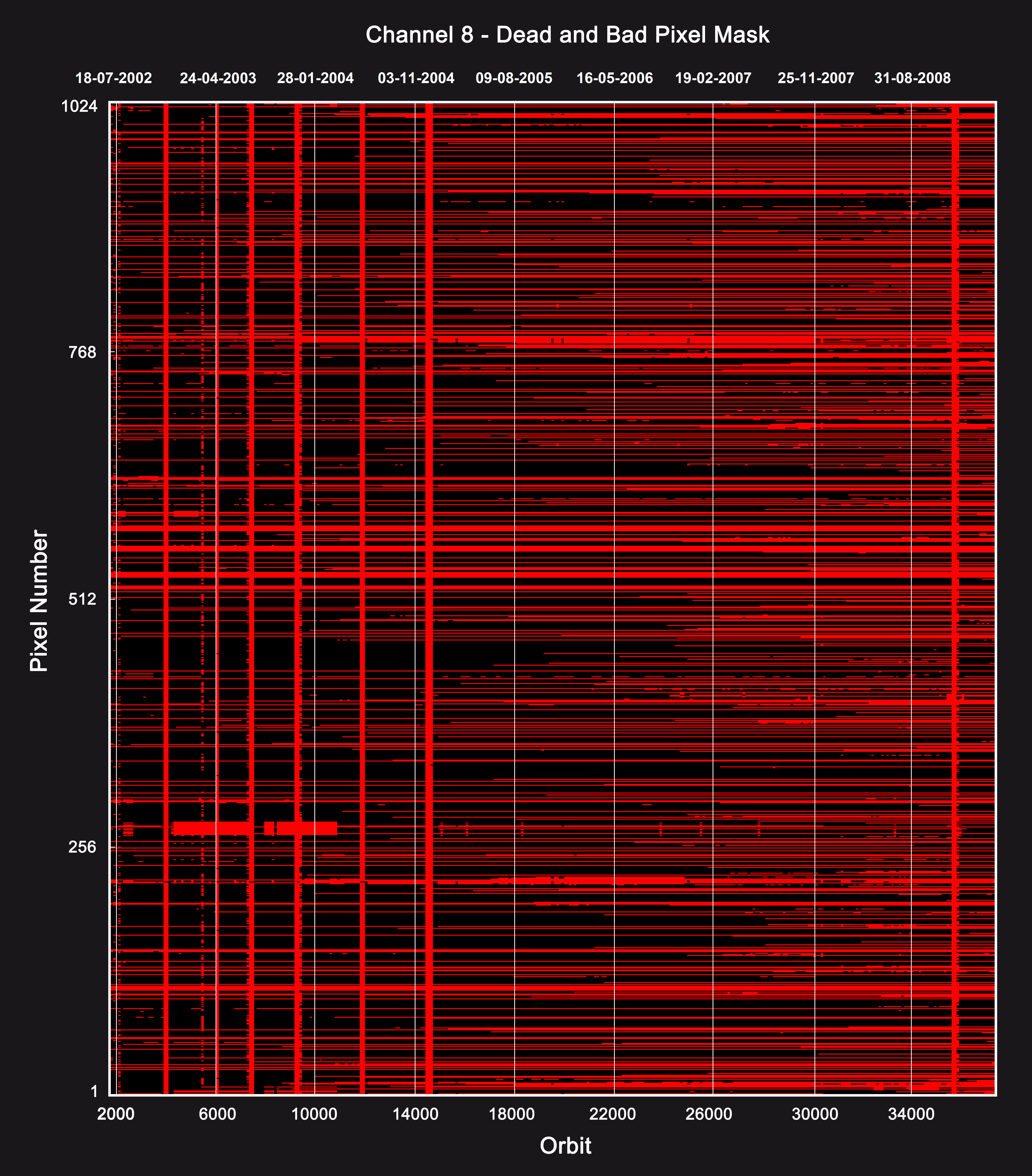
DBPM for channel 8 between August 2002 and March 2009. Each row corresponds to a single pixel.
When a pixel turns red it becomes either dead or bad. The vertical stripes correspond to decontamination periods.
(Courtesy: DLR-IMF)
|
|
| Fig. 8-7 |
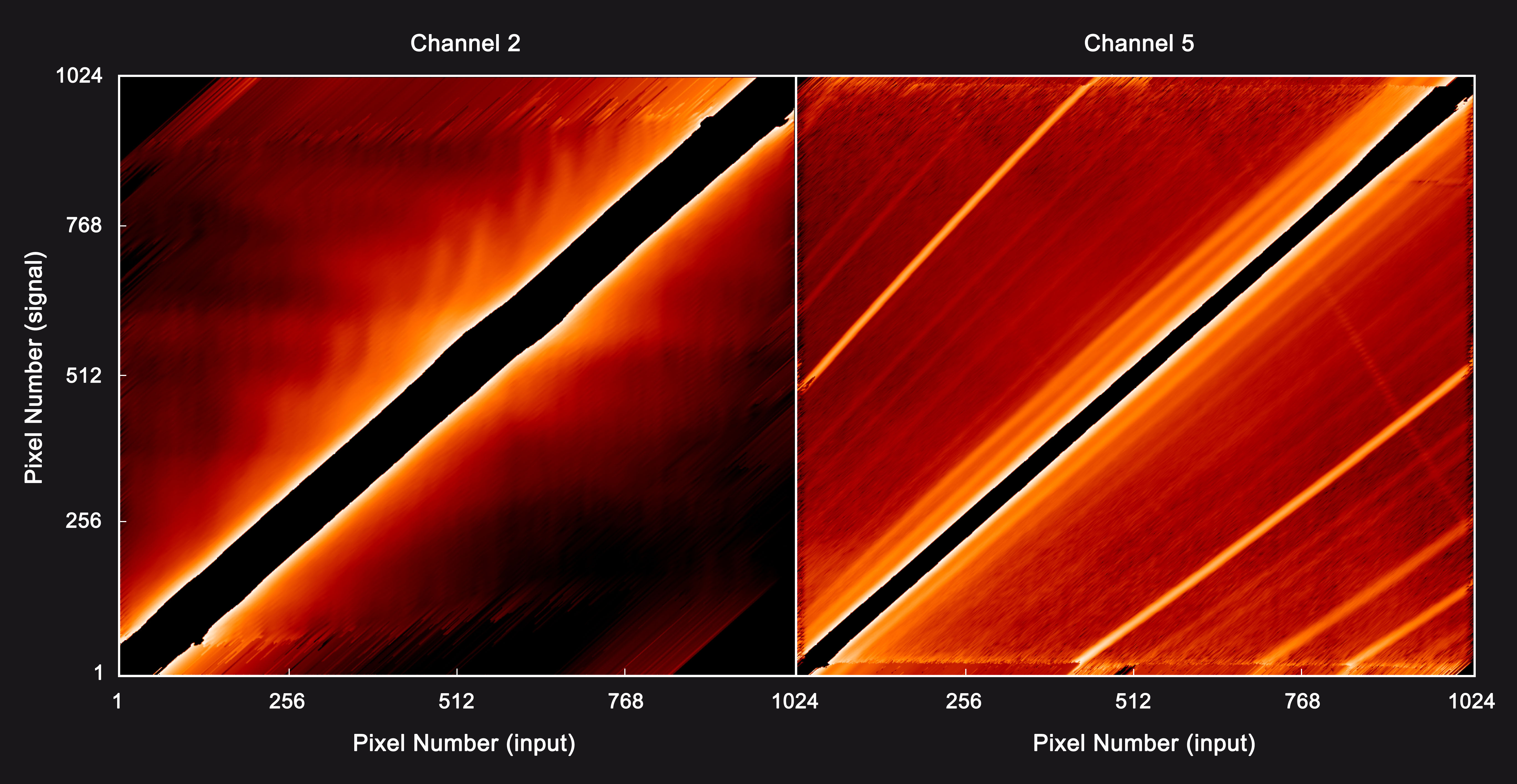
Spectral stray light matrix (1024 × 1024) in channel 2 (left) and channel 5 (right). Each row shows the
stray light spectrum (signal) due to unit input in the corresponding pixel (horizontal axis),
with bright regions displaying the strongest stray light contribution. The region around the diagonal
is defined as being free from stray light. The lines parallel and normal to the diagonal in the plot for
channel 5 are reflected and refocused ghosts. These are absent in channel 2, which has a holographic instead
of a classically ruled grating. (Courtesy: DLR-IMF)
|
|
| Fig. 8-8 |
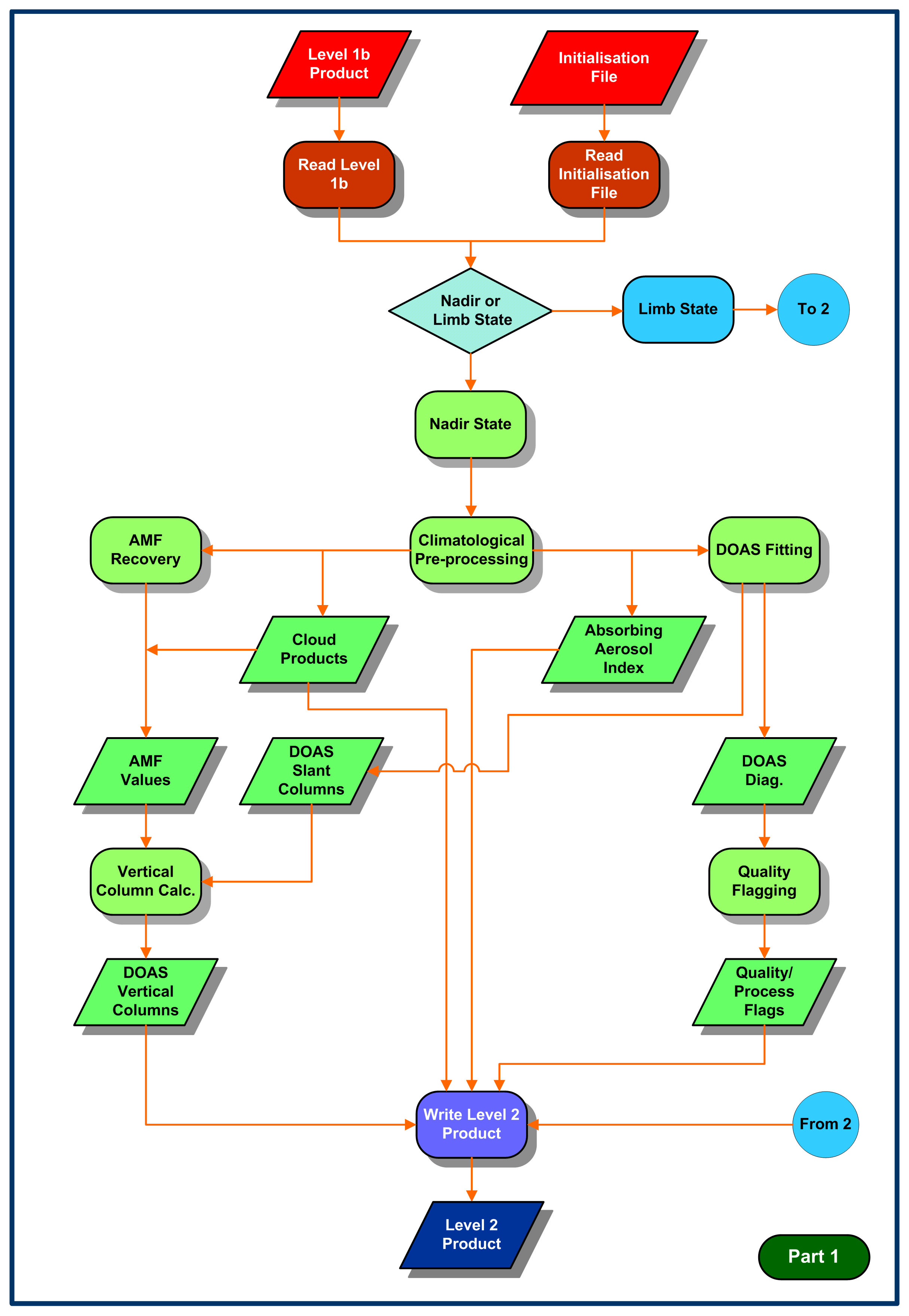
Level 1b-2 data processing flow diagram illustrating the preprocessing and nadir DOAS algorithm.
Limb algorithms are continued in Fig. 8-9. (Courtesy: DLR-IMF)
|
|
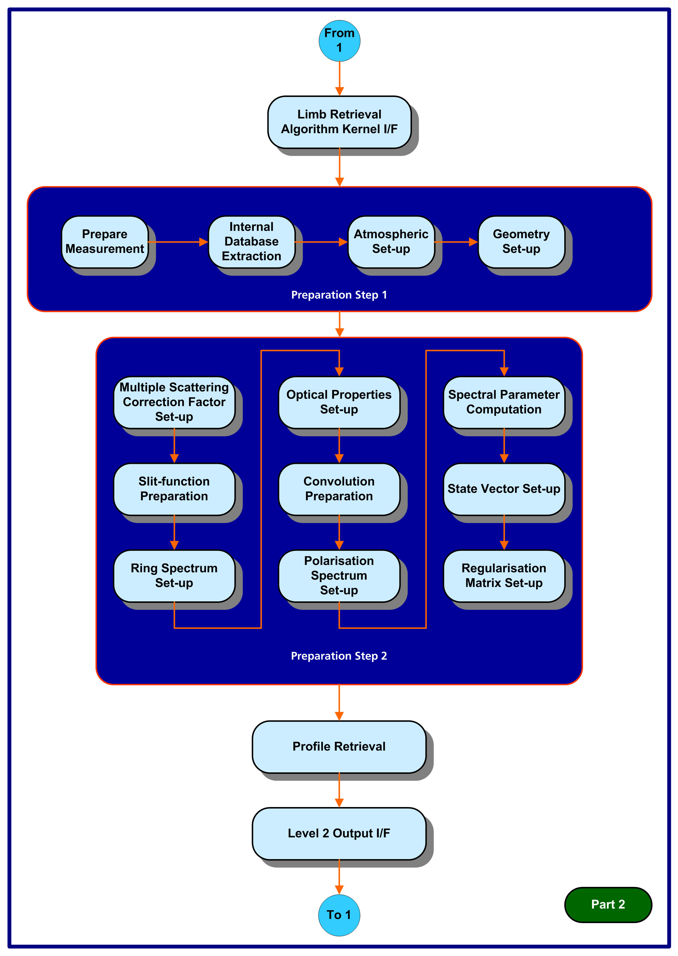
| Fig. 8-9 |
Level 1b-2 data processing flow diagram for limb profile retrieval. At the end of the limb processing, the
data flow returns to Fig. 8-8 for product output. (Courtesy: DLR-IMF)
|
|
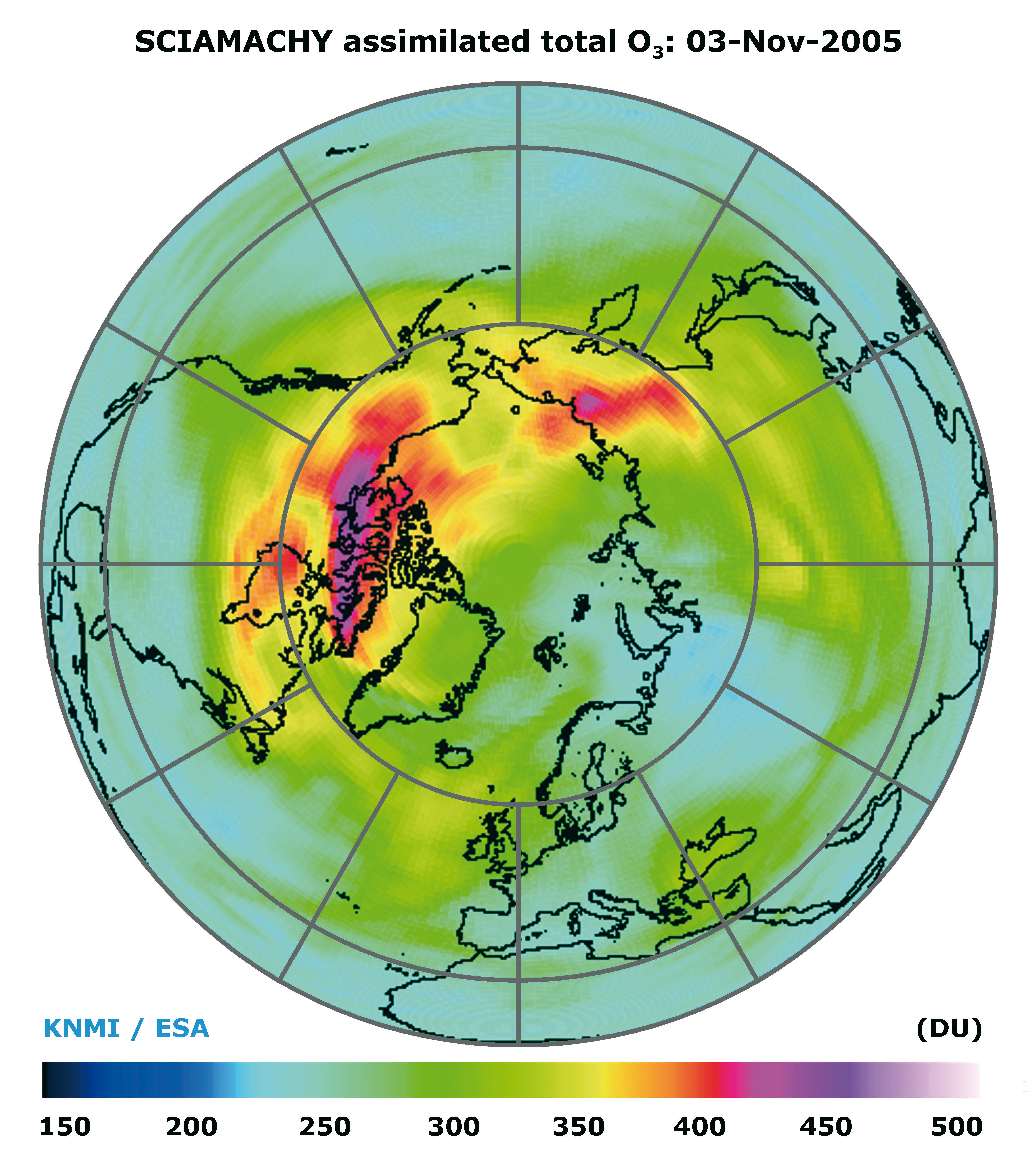
| Fig. 8-10 |
A forecasted North Pole view of the assimilated total ozone column field
for 3 November 2005 at 12:00 UTC based on SCIAMACHY data. (Courtesy: KNMI/ESA)
|
 |
Page generated 31 August 2011