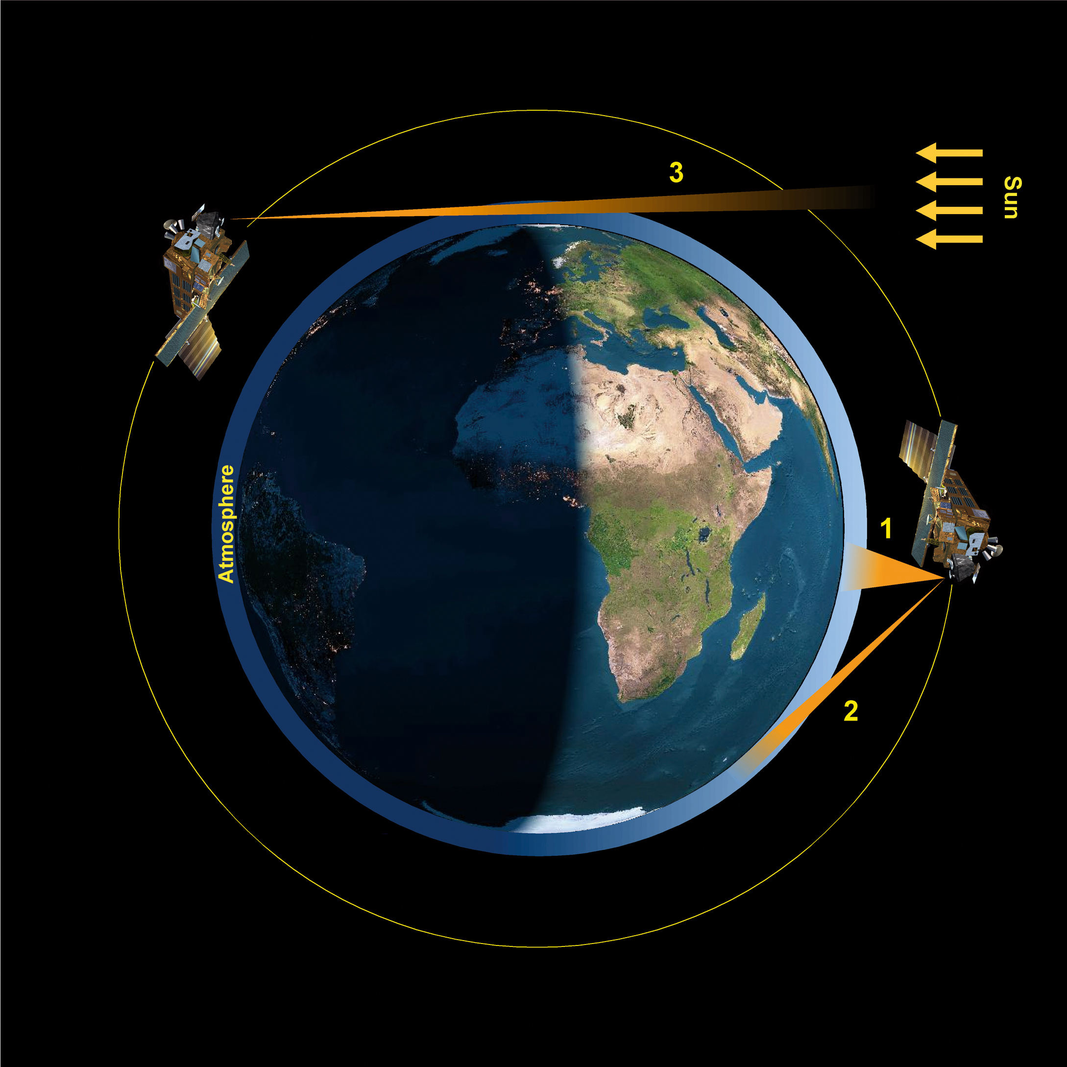
| Fig. 4-1 | SCIAMACHYs
scientific observation modes: 1 = nadir, 2 = limb, 3 = occultation.
(graphics: DLR-IMF) |
|
| Fig. 4-2 |
An orbit with planned limb/nadir matching on the dayside of the orbit.
The sequence of nadir and limb states in a timeline is arranged so that
limb ground pixels (blue), defined by the lineof- sight tangent point,
fall right into a nadir ground pixel (green). At the beginning and end
only limb or only nadir measurements are executed. (graphics: DLR-IMF)
|

|
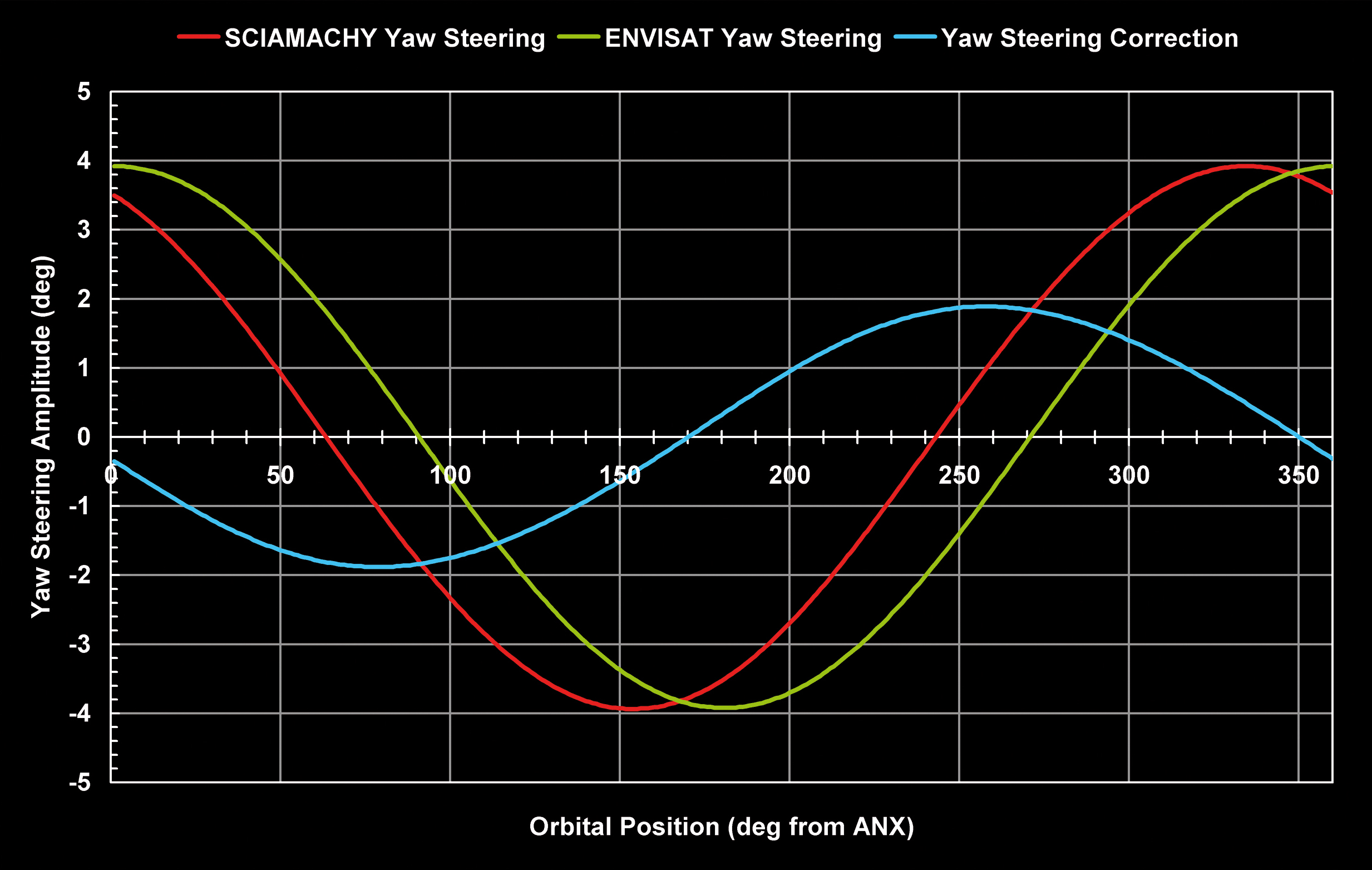
| Fig. 4-3 |
ENVISATs yaw steering, the yaw steering correction of limb states and
the resulting SCIAMACHY yaw steering. Between ENVISAT and SCIAMACHY
yaw steering an orbital shift of 27° exists which reflects the observation
geometry when looking to the horizon in flight direction. (graphics:
DLR-IMF) |
|
| Fig. 4-4 | SCIAMACHYs
monthly lunar visibility occurs between 1 and 2 over the southern hemisphere
(lunar phase > 0.5). The hatched area illustrates the limb TCFoV of
88°. Visibility at smaller lunar phases over the northern hemisphere
between 3 and 4 is not used because it coincides with solar occultation.
(graphics: DLR-IMF) |

|
| Fig. 4-5 |
The rising moon seen from a spacecraft in a low- Earth orbit. Differential
refraction distorts the lunar disk. (photo: NASA) |

|
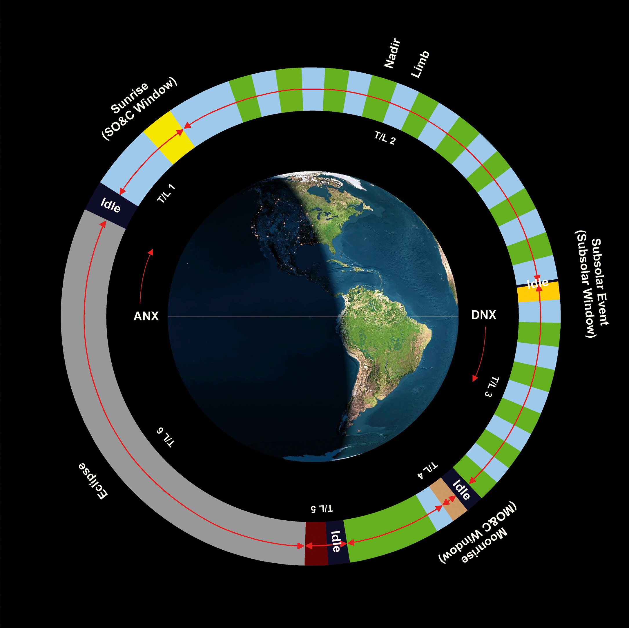
| Fig. 4-6 |
SCIAMACHY reference orbit with sun/moon fixed events along the orbit.
The events define orbital segments which are filled with timelines.
State duration is not to scale. (graphics: DLR-IMF) |
|
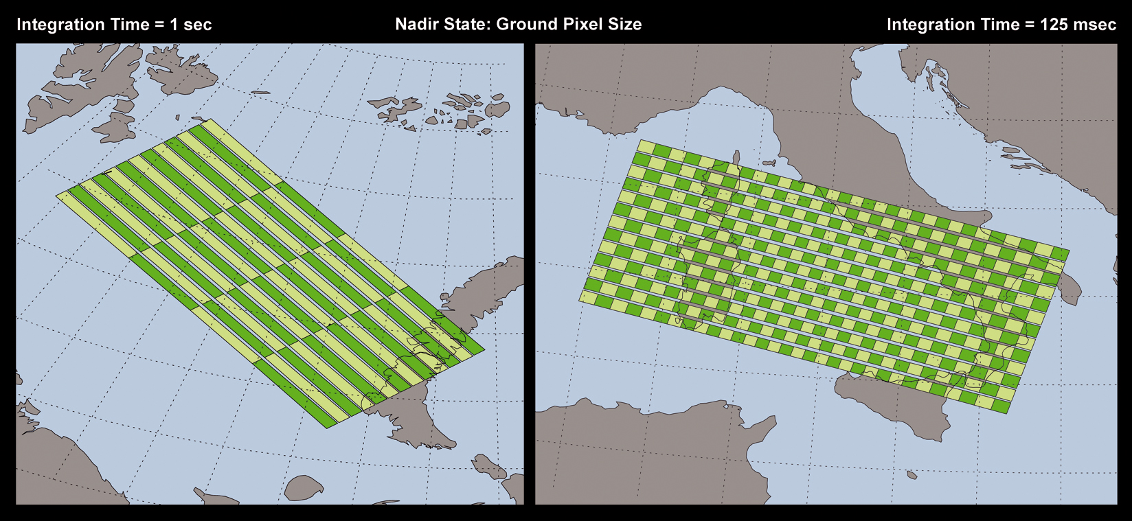
| Fig. 4-7 |
The pattern of ground pixels in a nadir measurement for an integration
time of 1 sec (left) and 125 msec (right). Only the forward scans are
shown. This causes the along-track gaps between consecutive scans which
vary in width due to a projection effect. Across-track extent is defined
by the integration time while along track the size reflects the dimension
of the IFoV with only a small contribution of the integration time.
(graphics: DLR-IMF) |
|
| Fig. 4-8 |
Calibration & monitoring scenarios from orbital to monthly timescales.
In the top row the individual measurements and their targets, e.g. sun,
moon, lamps, are listed. The states used in each calibration orbit,
referring to the definitions in table 4-2, are outlined below. All states
unrelated to the sun or the moon can be executed several times at any
position along the orbit. (graphics: DLR-IMF) |

|
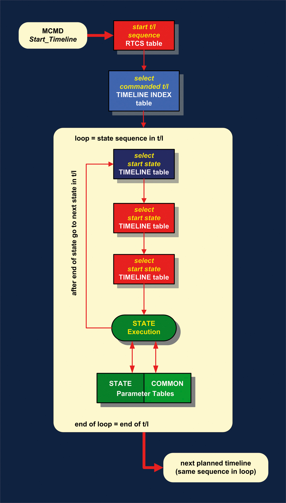
| Fig. 4-9 |
Information flow during timeline execution. Timelines are started by
macrocommand and end when the last state in the timeline has run to
completion. (graphics: DLRIMF) |
|
| Fig. 4-10 | Example
of the seasonal temporal variability of orbital segments. The time interval
between end of SO&C window and start of eclipse varies only slightly
over a year (yellow). In the monthly moon visibility periods, the time
between end of MO&C window and start of eclipse shows a much higher
variation (red curves). The blue segments indicate lunar visibility
phases where moonrise occurs on the nightside, i.e. those which can
be used for occultations. (graphics: DLR-IMF) |

|
Page generated 02 March 2007