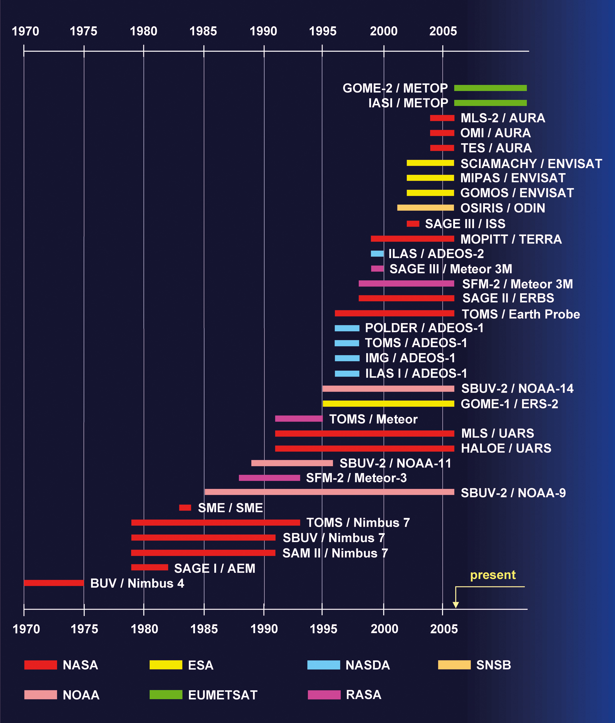
| Fig. 1-1 | Atmospheric
science spaceborne instruments and missions since 1970 with relevance
for SCIAMACHY. The list of missions is not intended to be complete but
to illustrate the progress in spaceborne instrumentation for atmospheric
composition monitoring. (graphics: DLR-IMF) |
|
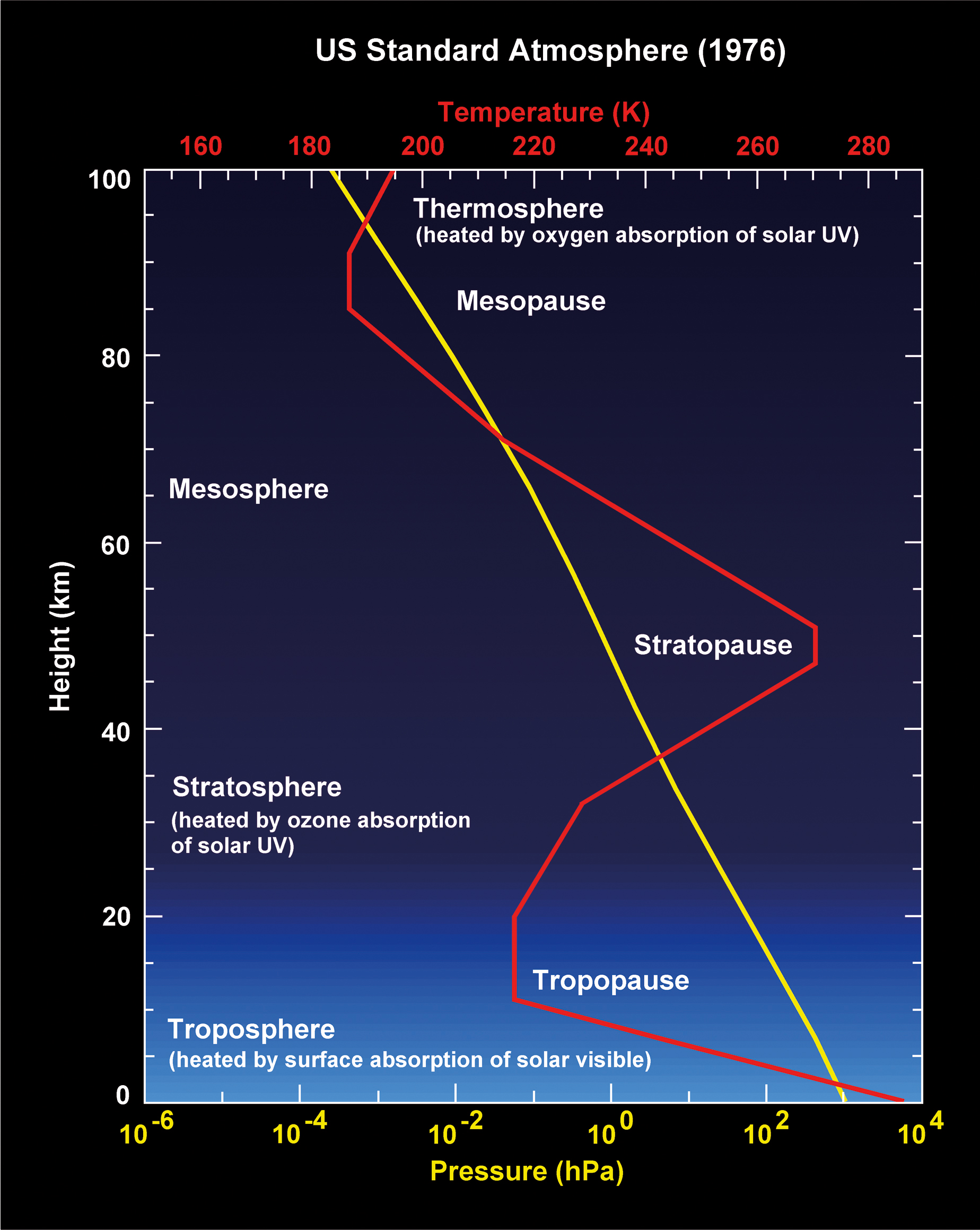
| Fig. 1-2 | Atmospheric
pressure and temperature profiles for mid latitudes (US Standard Atmosphere).
|
|
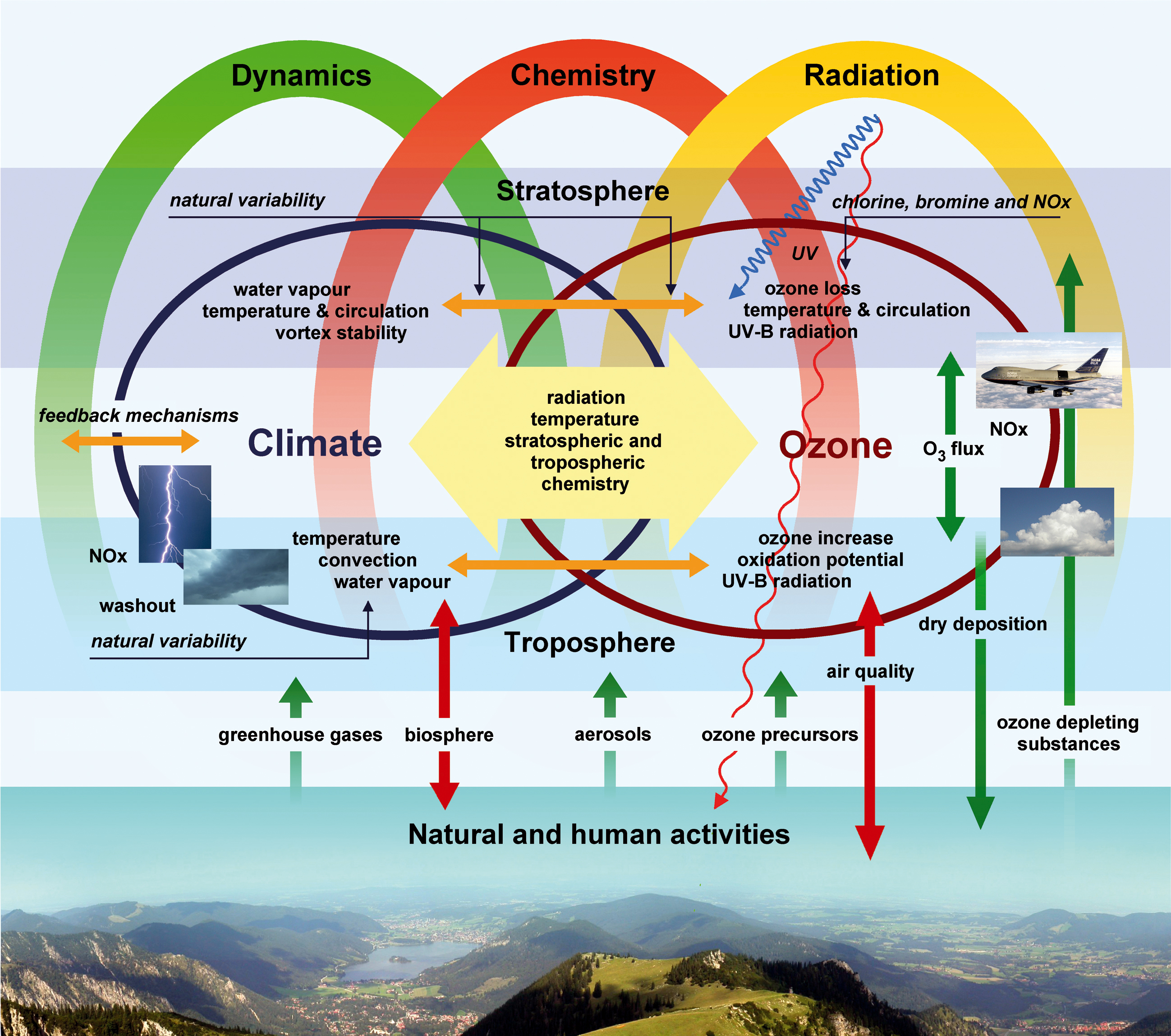
| Fig. 1-3 | Interactions
between human activity, atmospheric composition, chemical and physical
processes and climate. (graphics: DLR-IMF, after WMO-IGACO 2004)
|
|
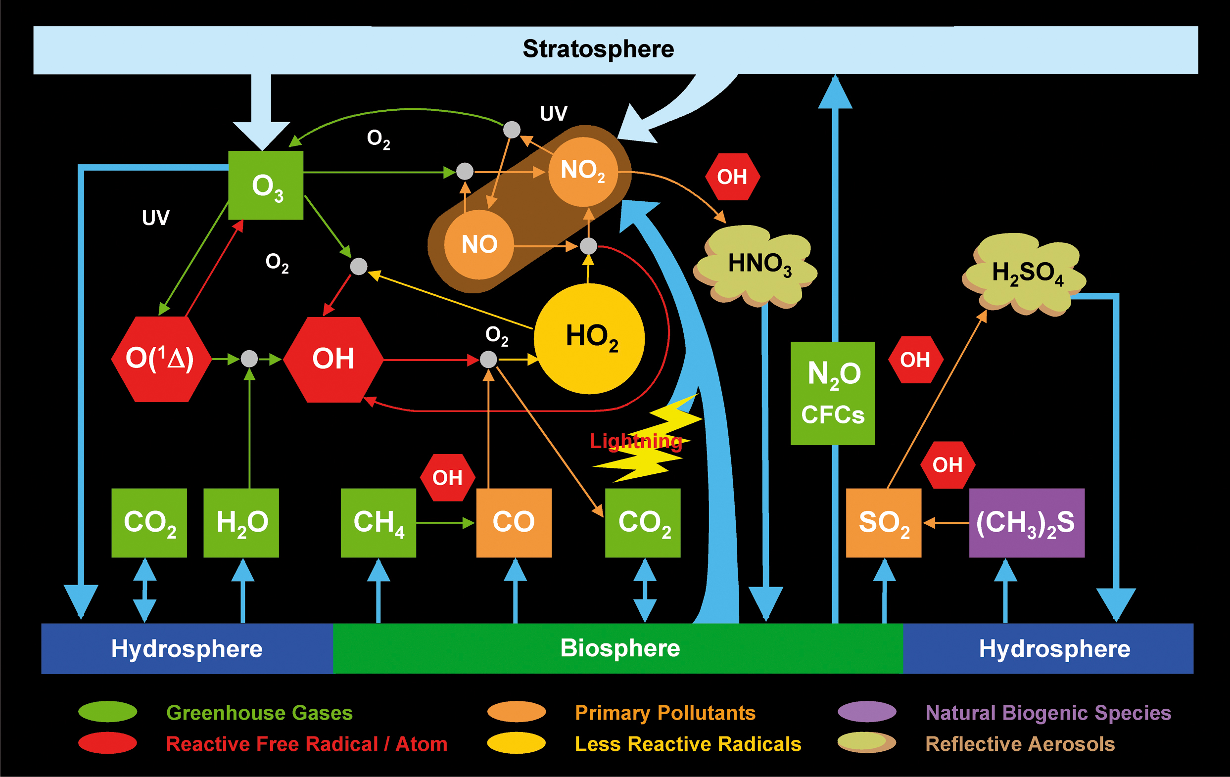
| Fig. 1-4 | The
dominant physical and chemical processes determining the composition
of the troposphere. (graphics: WMOIGACO 2004) |
|
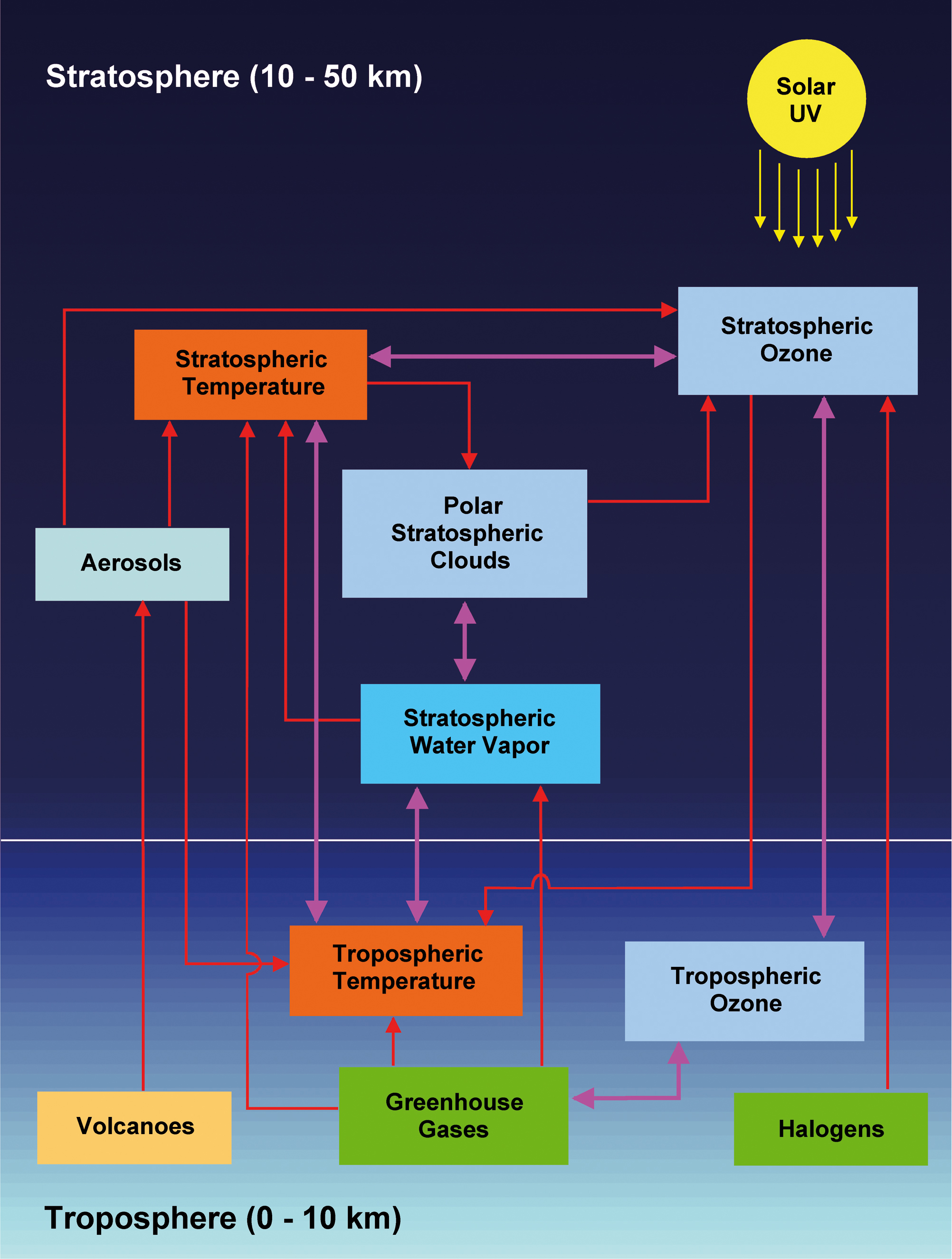
| Fig. 1-5 | Schematic
sketch of the interactions between stratospheric ozone and other atmospheric
constituents and processes. Anthropogenic emissions are shown in green
while other factors affecting the climate system (e.g., volcanoes) are
shown in beige. Red arrows indicate where one species or process affects
another. Feedbacks are shown with bold purple lines. For example, decreasing
polar stratospheric temperatures increase ozone depletion. Reduced ozone
then causes stratospheric cooling, creating a positive feedback. (graphics
after: NIWA) |
|
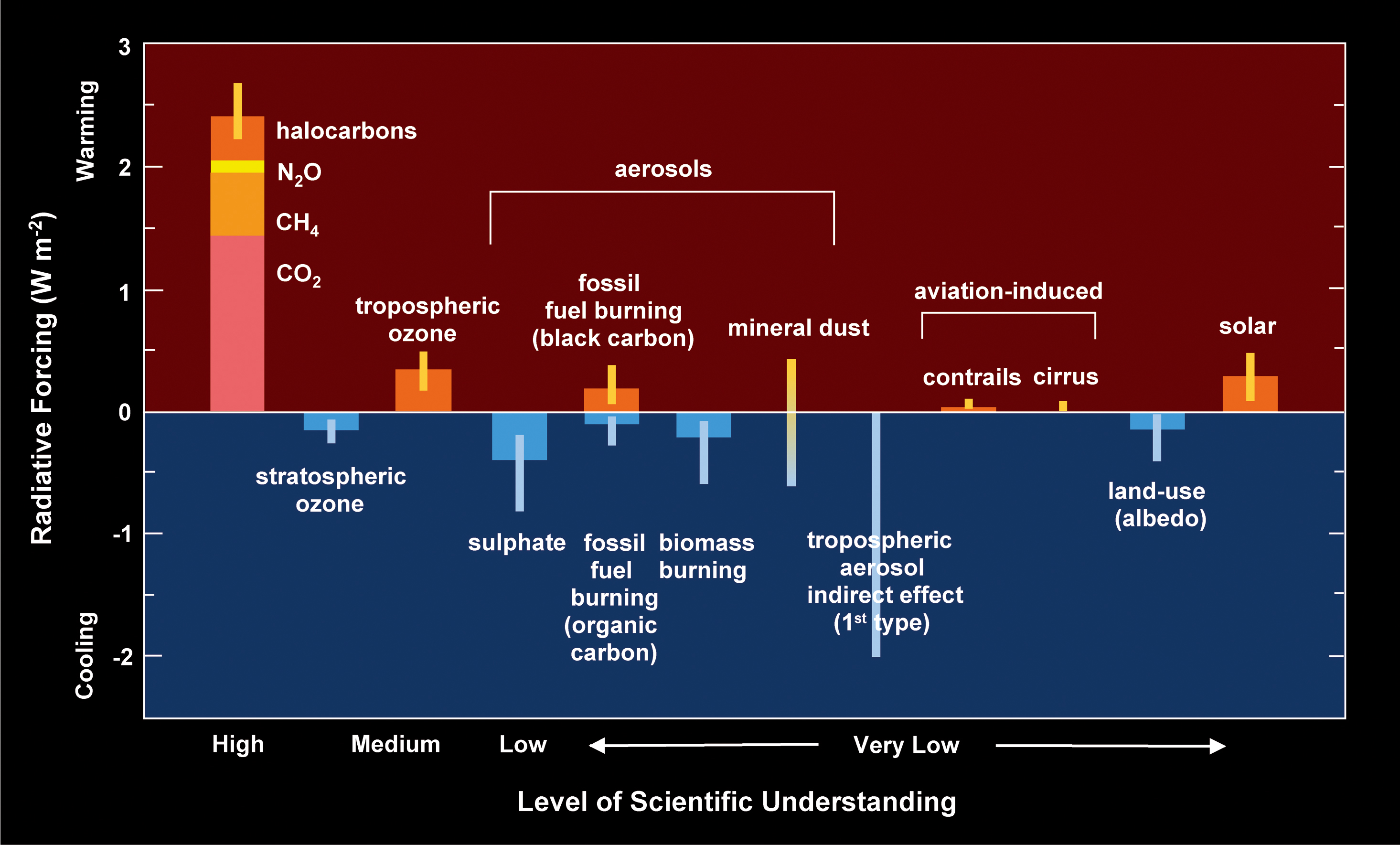
| Fig. 1-6 | Global,
annual mean radiative forcings (Wm-2) due to a number of agents for
the period from pre-industrial (1750) to present (late 1990s; about
2000). The height of each box denotes a central or best estimate value
while its absence indicates that no best estimate is possible. The vertical
bars visualise an estimate of the uncertainty range, for the most part
guided by the spread in the published values of the forcing. The uncertainty
range specified here has no statistical basis and therefore differs
from the use of the term elsewhere in this document. A level of scientific
understanding index is associated to each forcing, with high, medium,
low and very low levels, respectively. (IPCC 2001) |
|
Page generated 26 February 2007