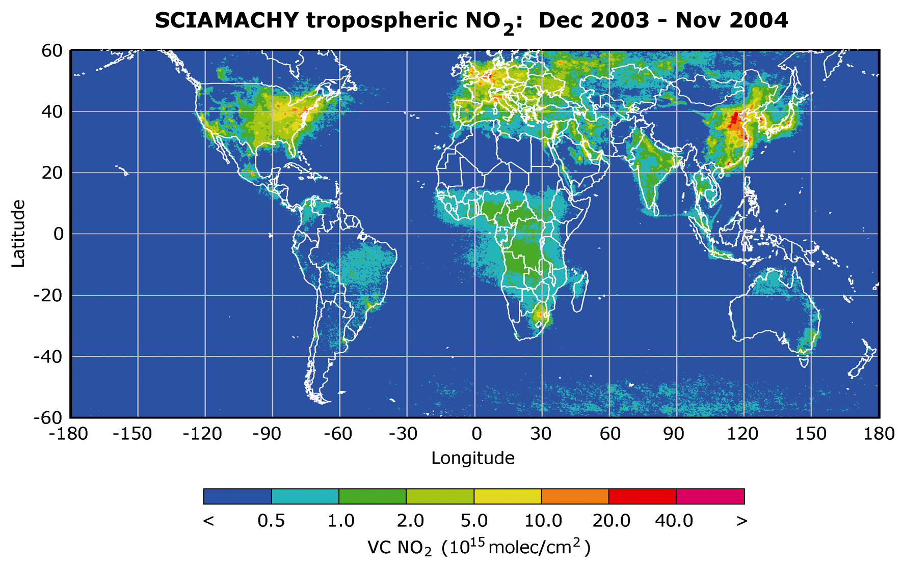
| Fig. 10-1 |
Global survey of tropospheric
NO2 for December 2003 to November 2004. Clearly visible are the industrialised
regions in the northern hemisphere and regions of biomass burning in
the southern hemisphere. (image: A. Richter, IUP-IFE,
University of Bremen) |
|
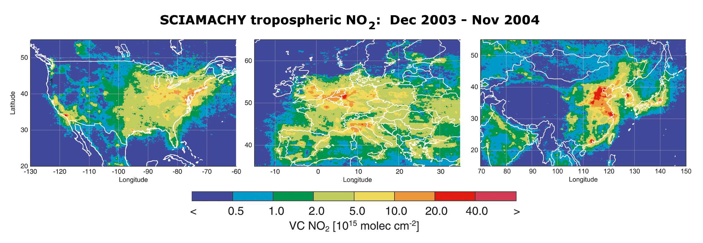
| Fig. 10-2 | Mean
tropospheric NO2 densities over Europe, the United States and China
between December 2003 and November 2004. (image: A. Richter, IUP-IFE, University of Bremen) |
|
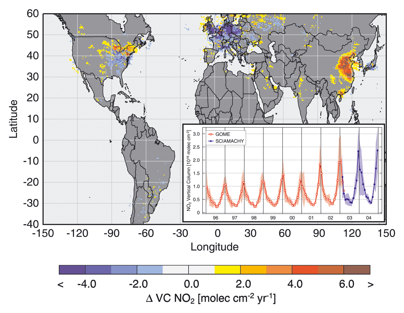
| Fig. 10-3 | Change
in global tropospheric NO2 concentrations from 1996-2002. The inset illustrates
how NO2 concentrations have risen in China from 1996-2004. The trend analysis uses
data from GOME (1996-2002) and SCIAMACHY (2003-2004). While 'old'; industrialised countries
were able to stop the increase of NO2 emissions, the economical growth in China
turns out to be a strong driver for pollution. (image: A. Richter, IUP-IFE, University of Bremen) |
|
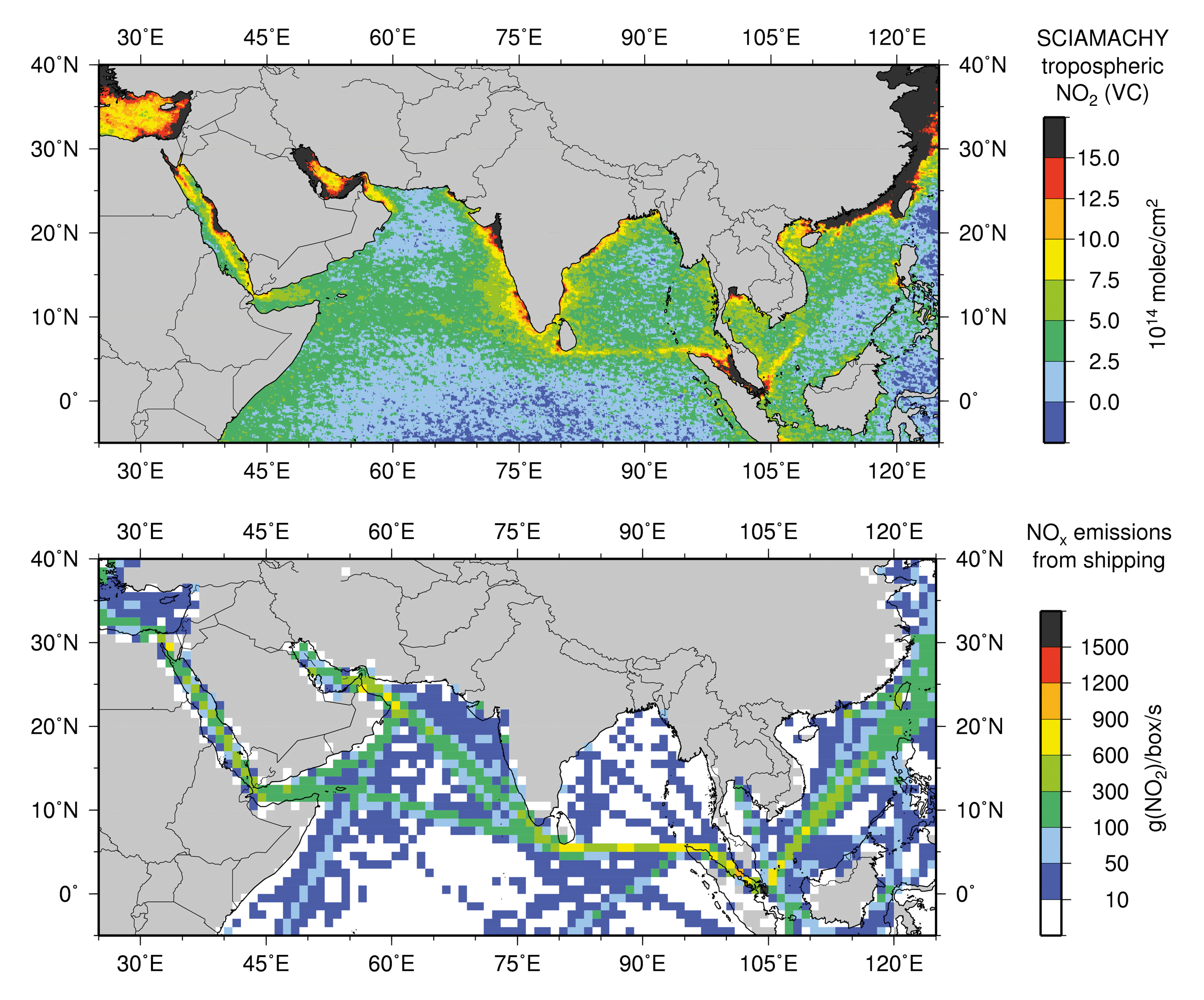
| Fig. 10-4 | NO2
densities over the Indian Ocean and the Red Sea as derived from measurements
between August 2002 and April 2004 (top). The highly frequented ship routes from Eastern Asia
to the Suez Canal can be clearly seen. Along the coast lines strong NO2 concentrations are the result of urban industrialised
areas. In the lower panel the NOx emissions associated with shipping based on emission inventories is depicted. (image: A.
Richter, IUP-IFE, University of Bremen) |
|
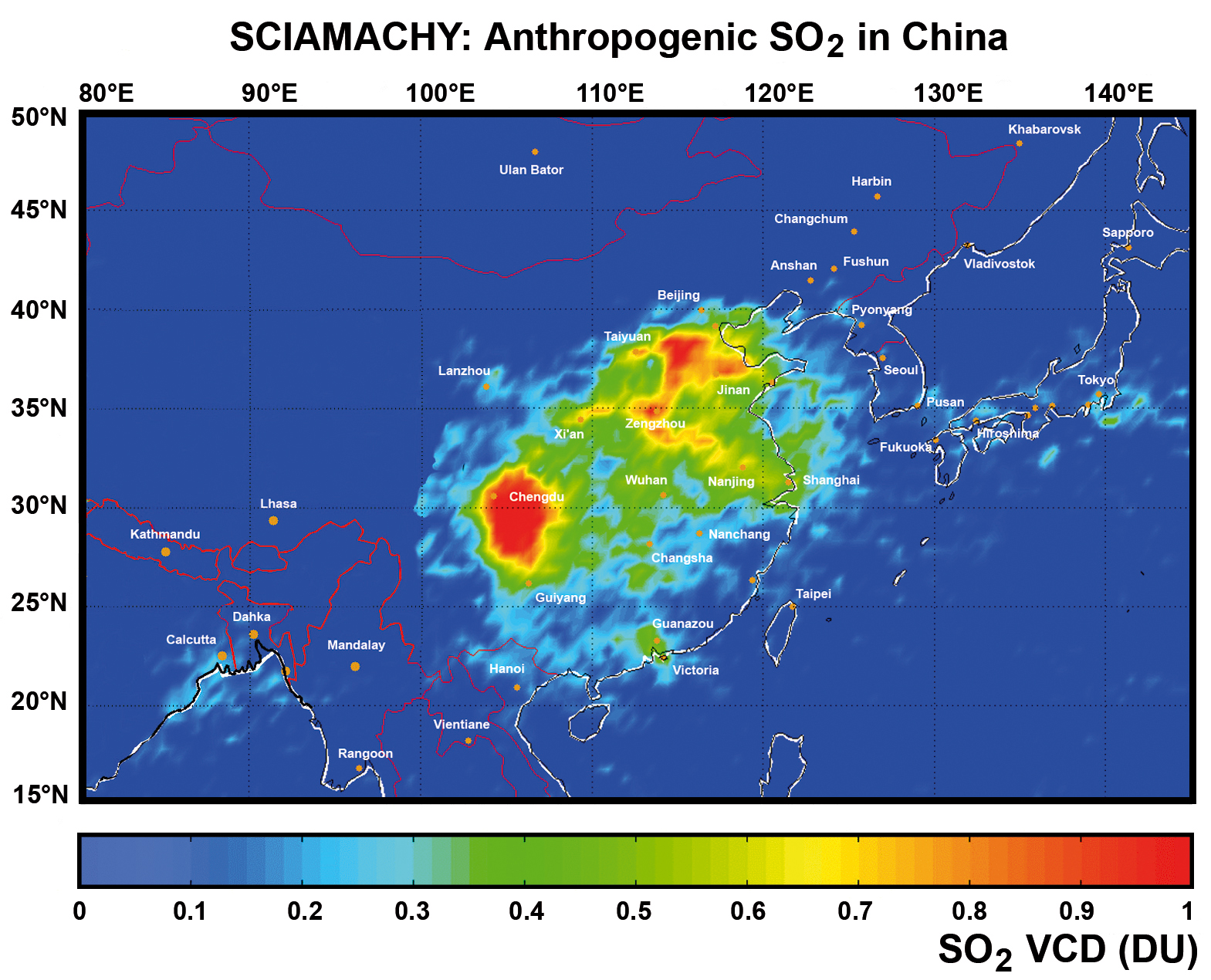
| Fig. 10-5 | Average
SO2 column densities over eastern China during the year 2003. SCIAMACHY's
improved spatial resolution permits to identify localised emissions due to anthropogenic
activities. (image: M.Van Roozendael, IASB-BIRA) |
|
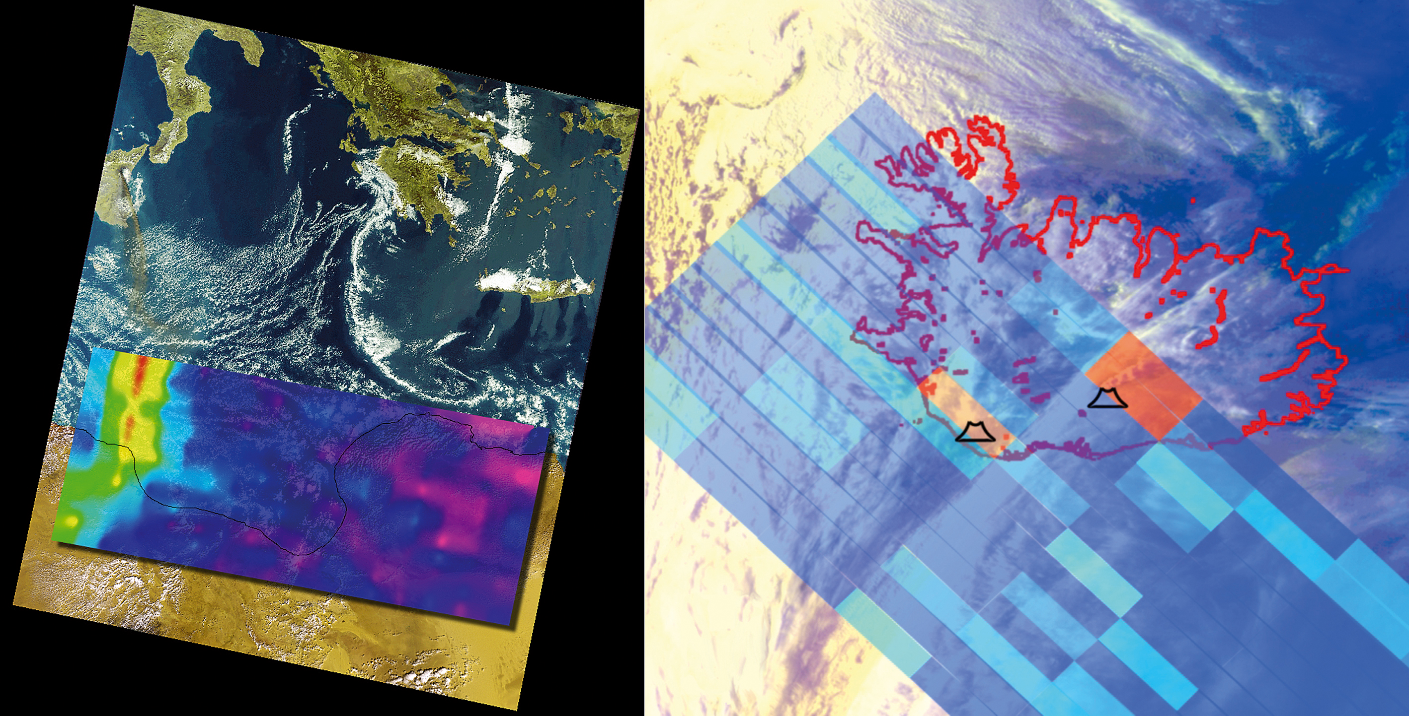
| Fig. 10-6 | Two
European volcanic eruptions with obvious SO2 emissions: Mt. Etna (left)
and Grimsvötn (right). The SCIAMACHY nadir measurement of Mt. Etna is overlayed on a MERIS image showing
that the plumes of SO2 and visible ash match well. In the Iceland image (right) detected SO2 emission at Grimsvötn
is indicated by the red pixel. The second faint SO2 enhancement in the south of Iceland is caused by the Katla volcanoe.
The underlying visible image stems from AVHRR/NOAA-12. (images: Mt. Etna – DLR-IMF, Iceland – DLR-DFD
and IUP-IFE, University of Bremen) |
 |
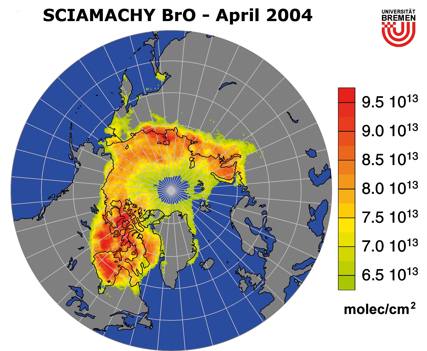
| Fig. 10-7 | BrO
concentrations over the arctic sea ice in April 2004. (image: DLR-DFD and IUP-IFE, University of Bremen) |
|
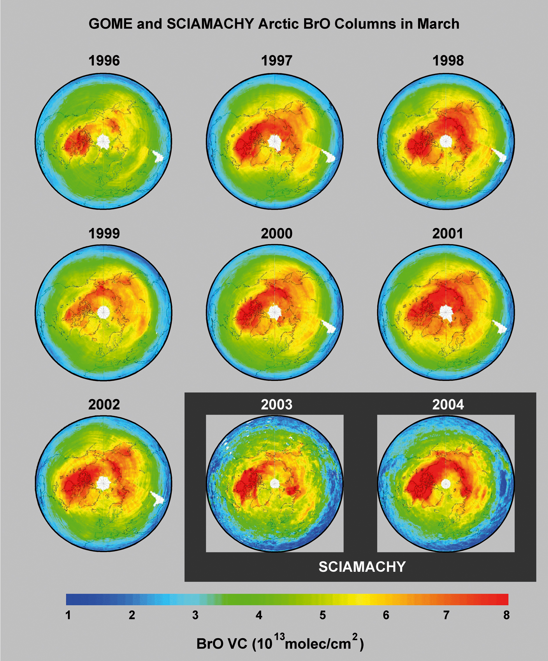
| Fig. 10-8 | A
long-term study of BrO concentrations over the arctic ocean in March
from 1996-2004 using data from GOME and SCIAMACHY. (images: M. Van Roozendael, BIRA) |
|
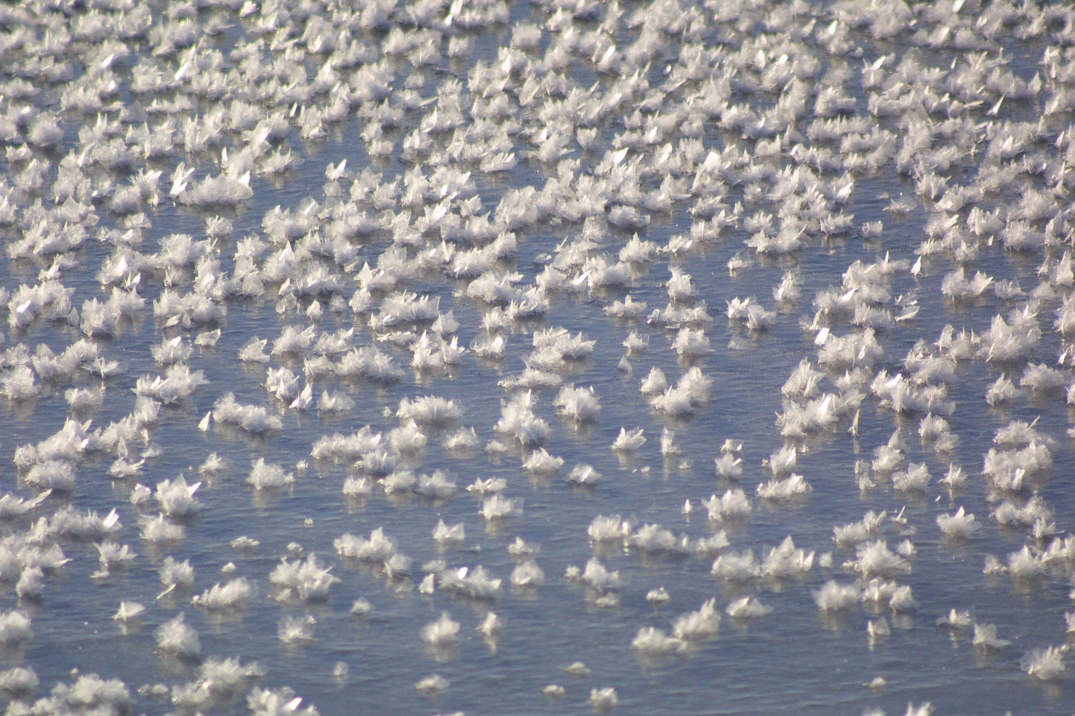
| Fig. 10-9 | Frost
flowers on the surface of water. They contain bromine which is released
when the flowers begin to vanish at the end of the arctic winter. (photo: S. Kern, University of Hamburg) |
|
| Fig. 10-10 | The
global distribution of formaldehyde (HCHO), derived from SCIAMACHY measurements
from August 2004 to July 2005. In the SAA data analysis is of reduced quality.
(image: F. Wittrock, IUP-IFE, University of Bremen) |
 |
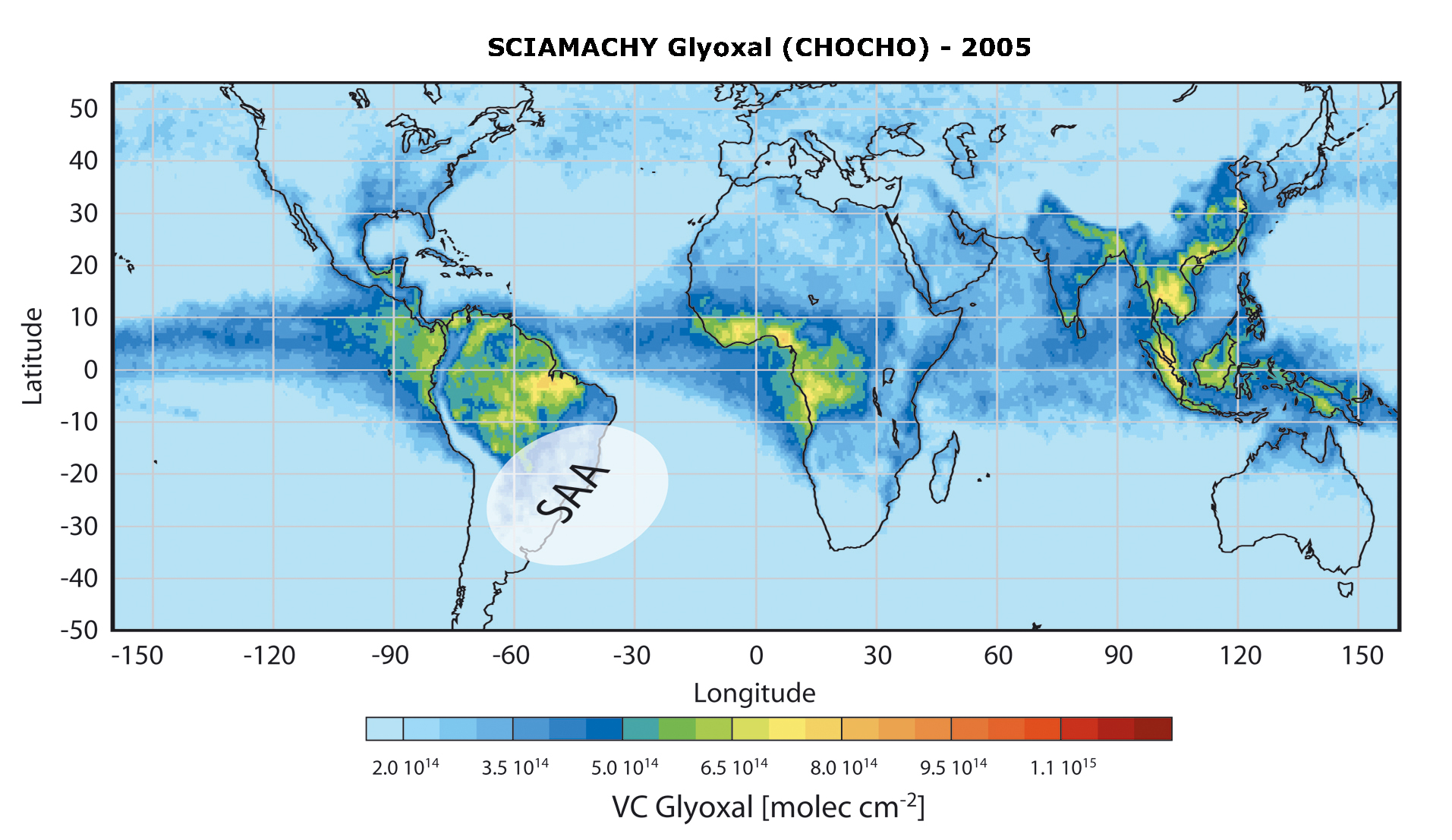
| Fig. 10-11 | The
global distribution of glyoxal (CHOCHO) for the year 2005, as derived
from SCIAMACHY measurements. In contrast to formaldehyde, direct emissions of glyoxal are believed to
be small and therefore glyoxal is a better indicator for VOC oxidation, the main source of photochemical smog. In the SAA data
analysis is of reduced quality. (image: F. Wittrock, IUP-IFE, University of Bremen) |
|
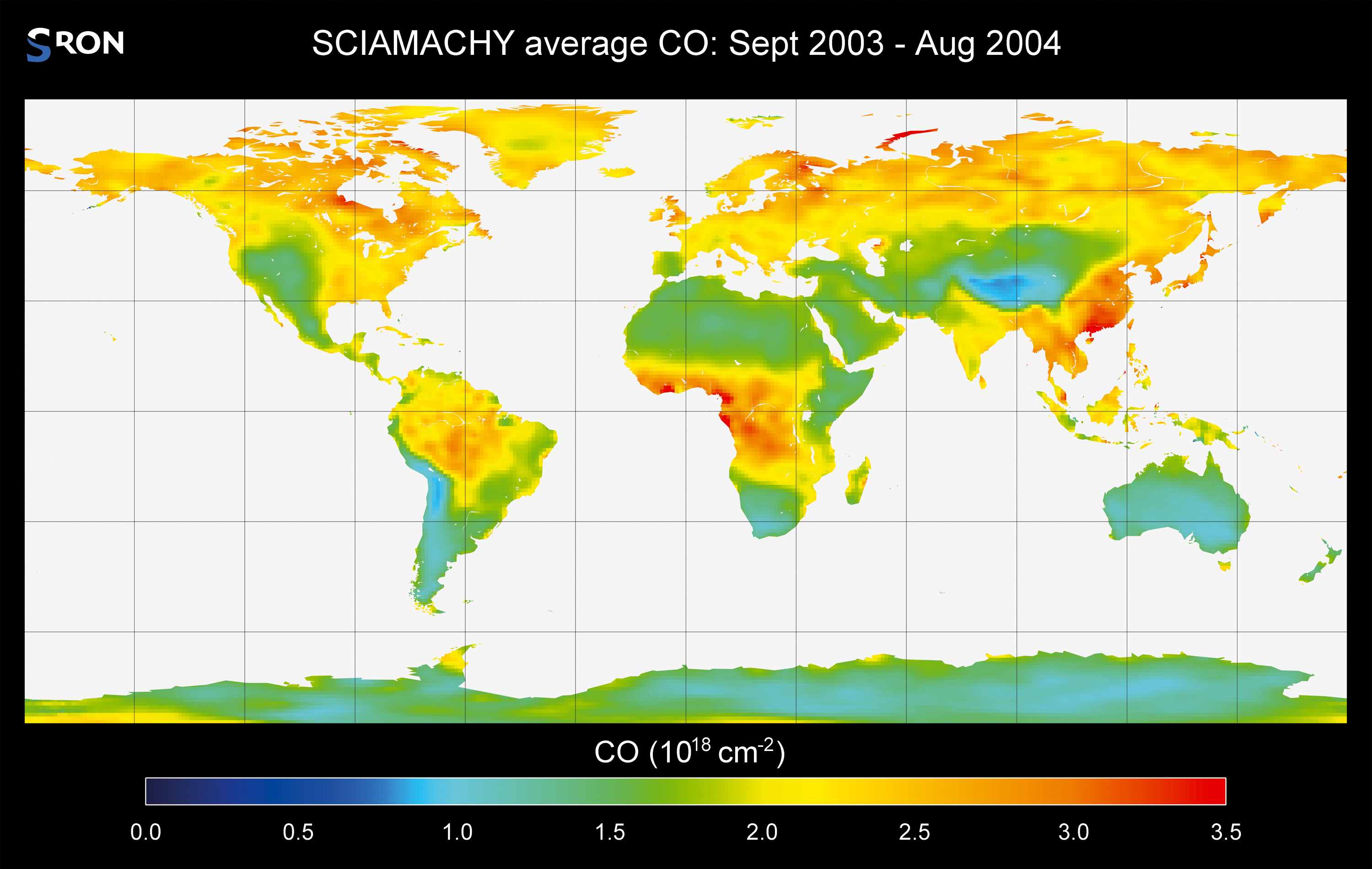
| Fig. 10-12 | The
global distribution of carbon monoxide. Elevated CO is present in regions
with biomass burning. The data is largely consistent with MOPITT and model results. (image: H. Schrijver, SRON) |
|
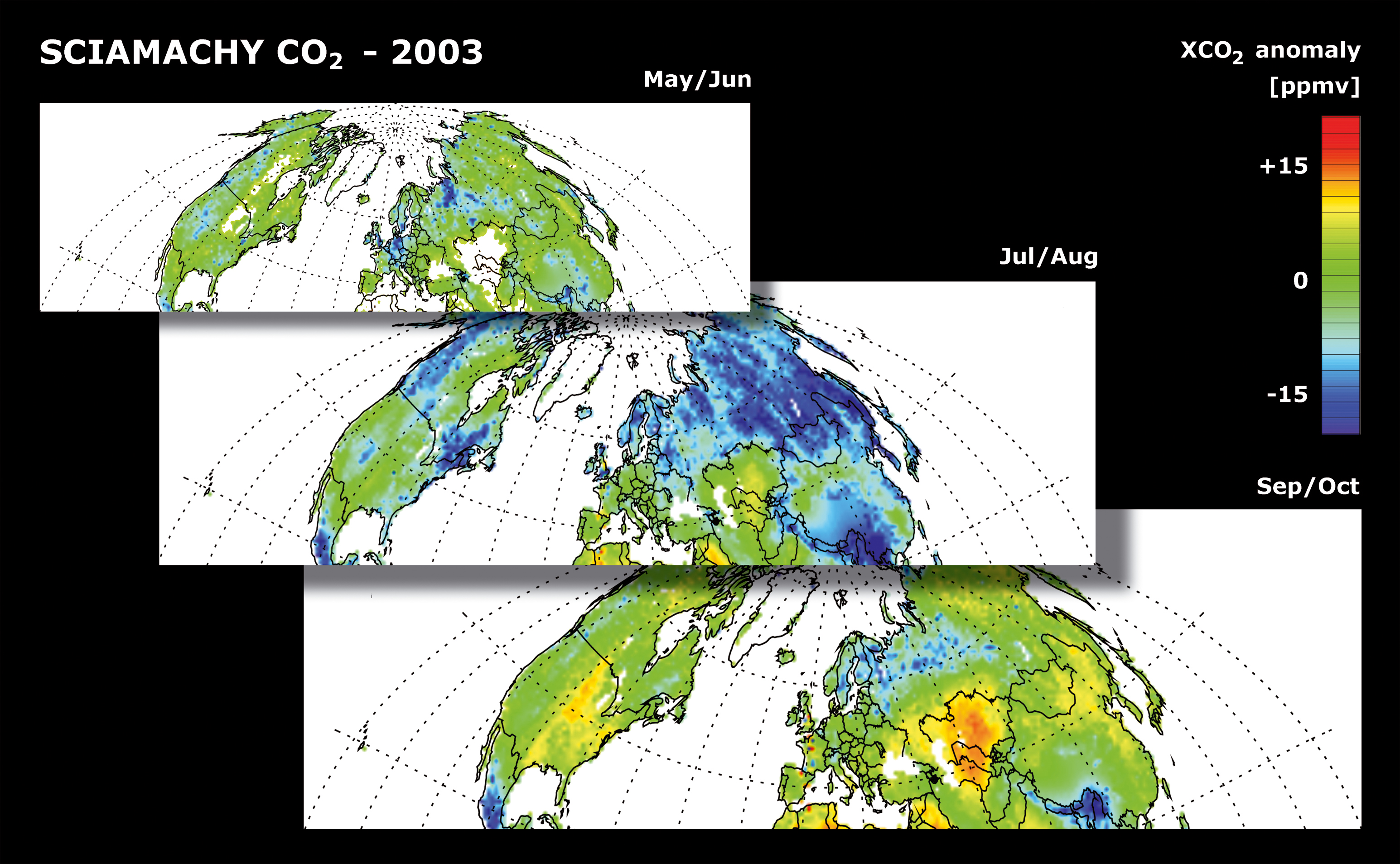
| Fig. 10-13 | Atmospheric
CO2 as measured by SCIAMACHY over the northern hemisphere during the
year 2003. Low values (blue) during July/August compared to higher values (green and yellow)
before and after this time period are due to uptake of atmospheric CO2 by vegetation, e.g. boreal forests, which is in its
growing phase during the summer months. (image: M. Buchwitz, IUP-IFE, University of Bremen) |
|
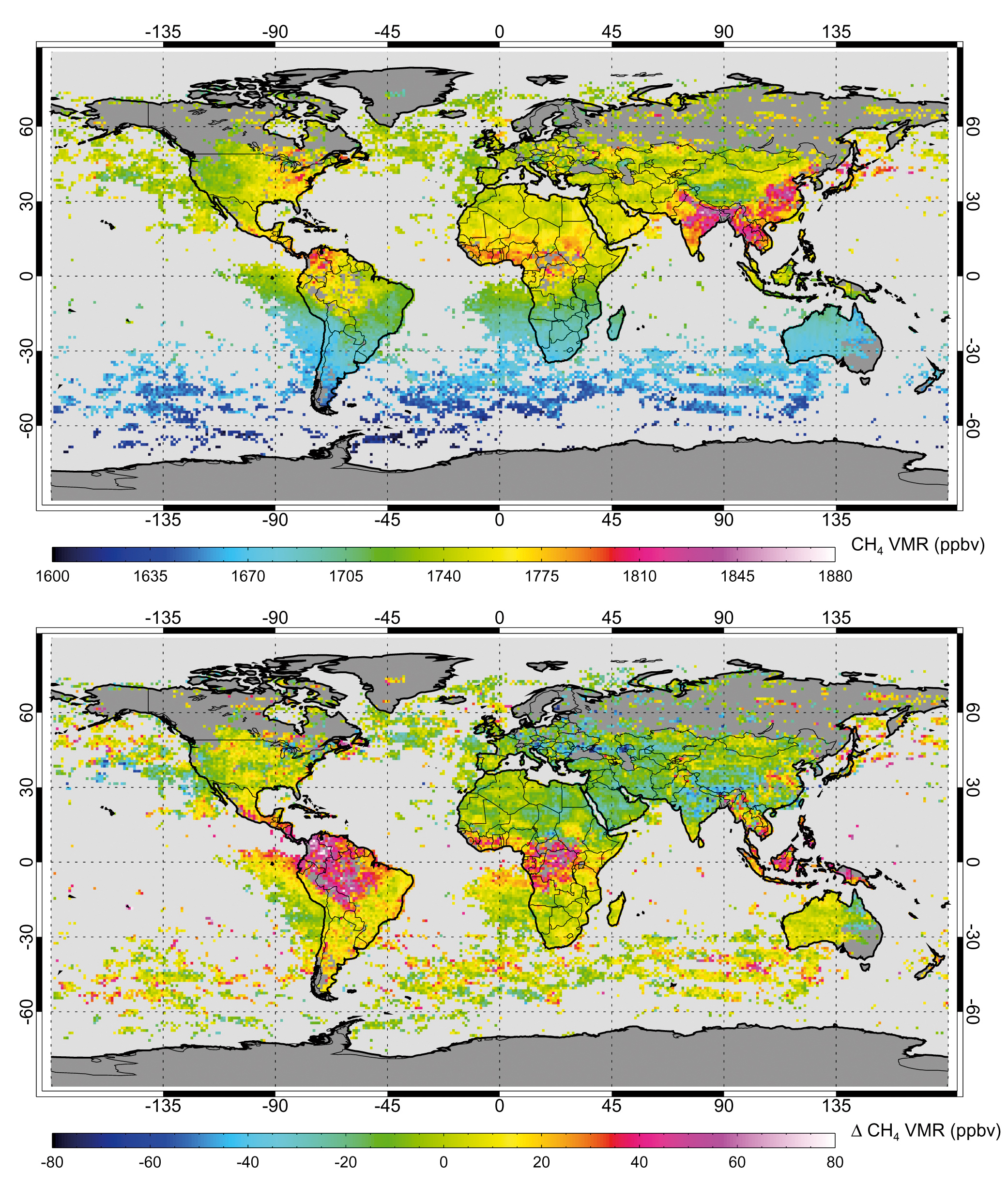
| Fig. 10-14 | Methane
concentrations for August-November 2003 (top). Emissions are high in
India and parts of China due to agricultural activities but also over tropical rainforests with still
unknown reason. This phenomenon becomes obvious when measurements are compared with model calculations. In the bottom panel
the difference between retrieved and modelled densities is shown with discrepancy 'hot spots' in Indonesia,
Central Africa and South America. (images: Frankenberg et al. 2005) |
|
| Fig. 10-15 | Global
monthly mean of gridded SCIAMACHY water vapour columns for October 2003.
White areas denote either regions of missing SCIAMACHY data or high mountain areas where data
have been removed by the inherent AMC-DOAS quality check. (image: S. Noël, IUP-IFE, University of Bremen) |

|
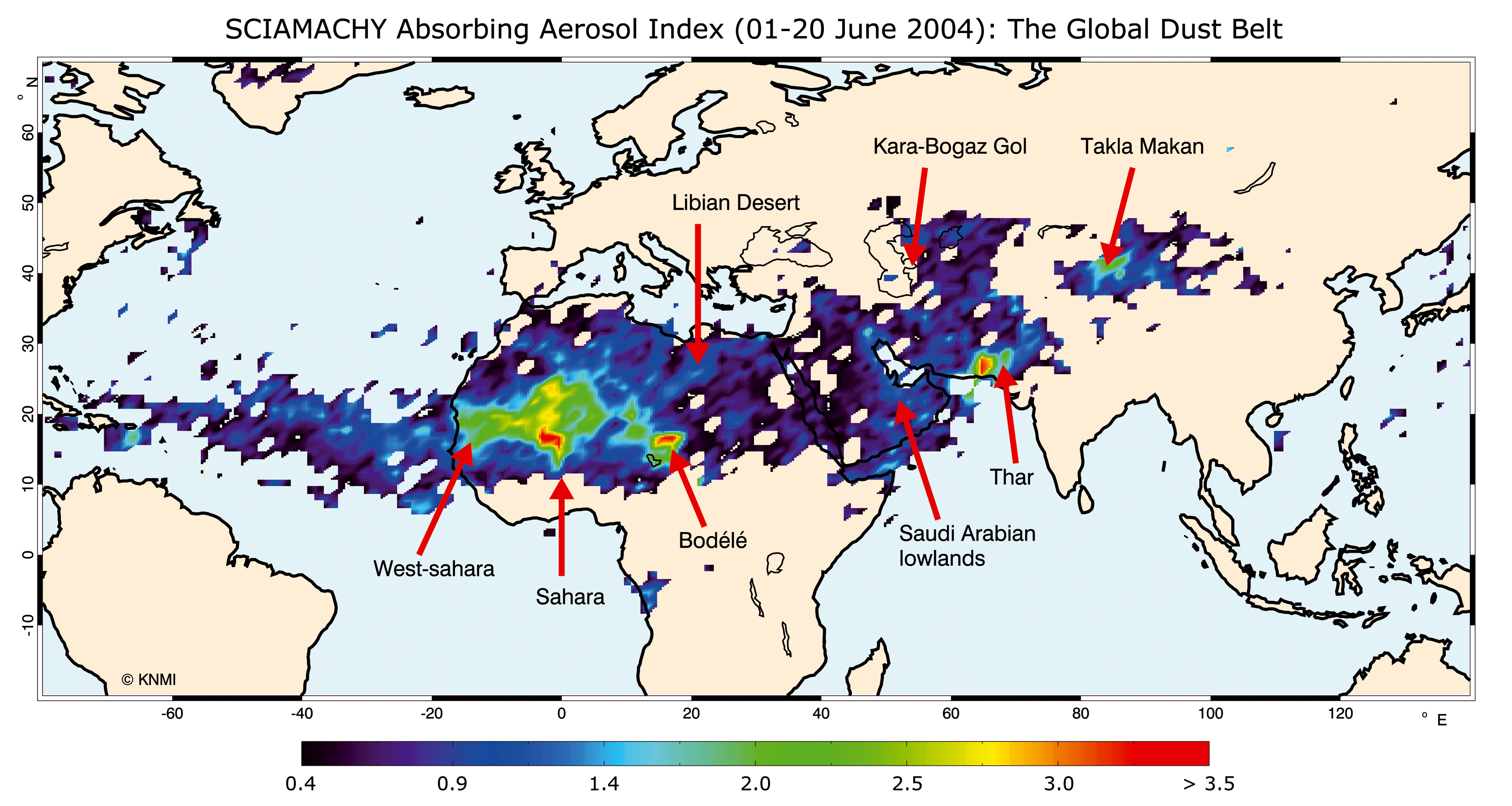
| Fig. 10-16 | The
Global Dust Belt. A 20 day average of SCIAMACHY AAI in June 2004 shows the spatial distribution of desert
dust, called the Global Dust Belt (Prospero et al. 2002). Even from a 20 day average, AAI peaks coincide with the major
desert areas in the northern hemisphere and the AAI shows Saharan dust being transported over the Atlantic Ocean. (image:
M. de Graaf, KNMI) |
|
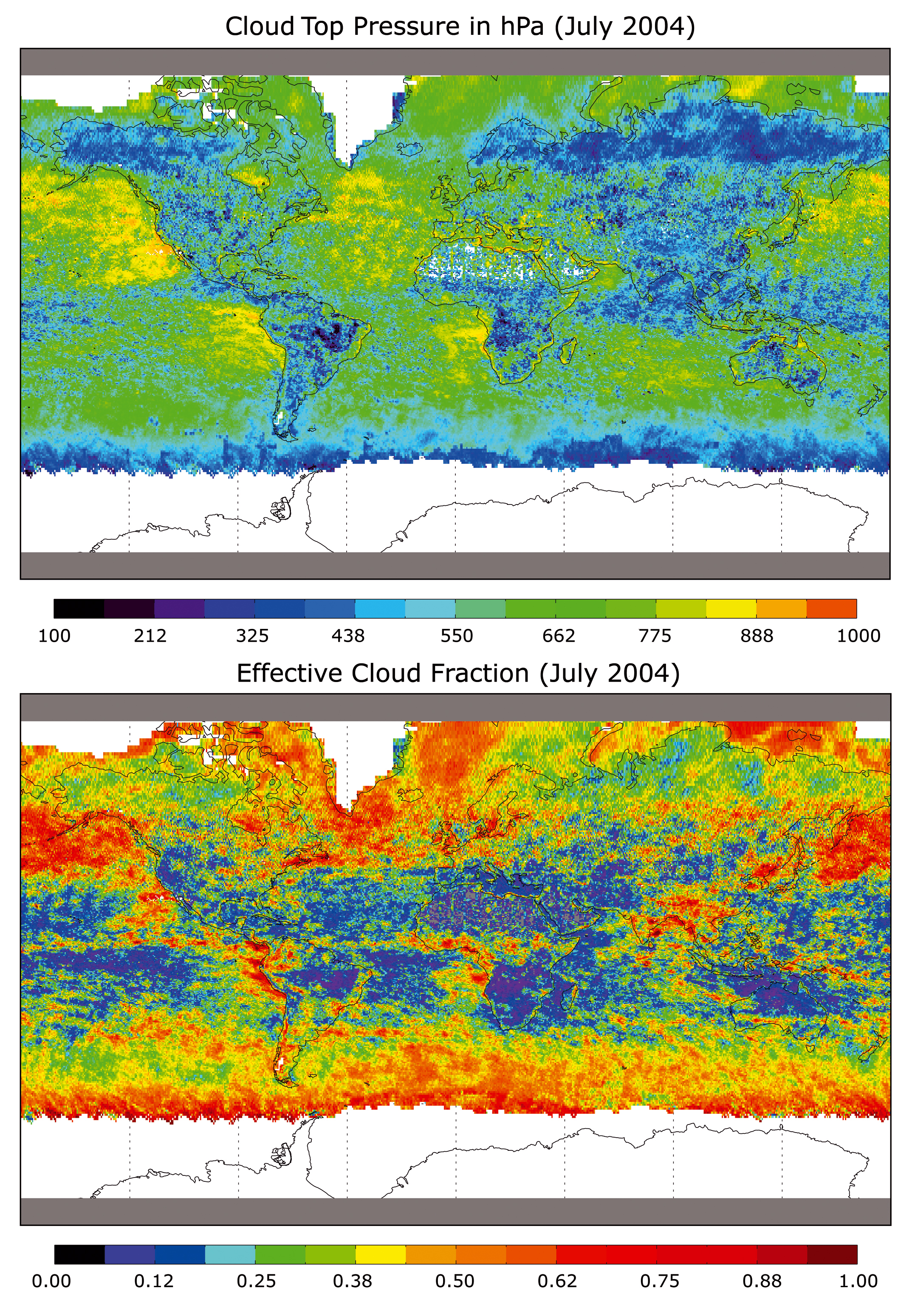
| Fig. 10-17 | Examples
of global maps of SCIAMACHY O2 A-band cloud results from the FRESCO
algorithm: Effective cloud top pressure for July 2004 (top) and effective cloud fraction for July
2004 (bottom). (images: KNMI/ESA) |
|
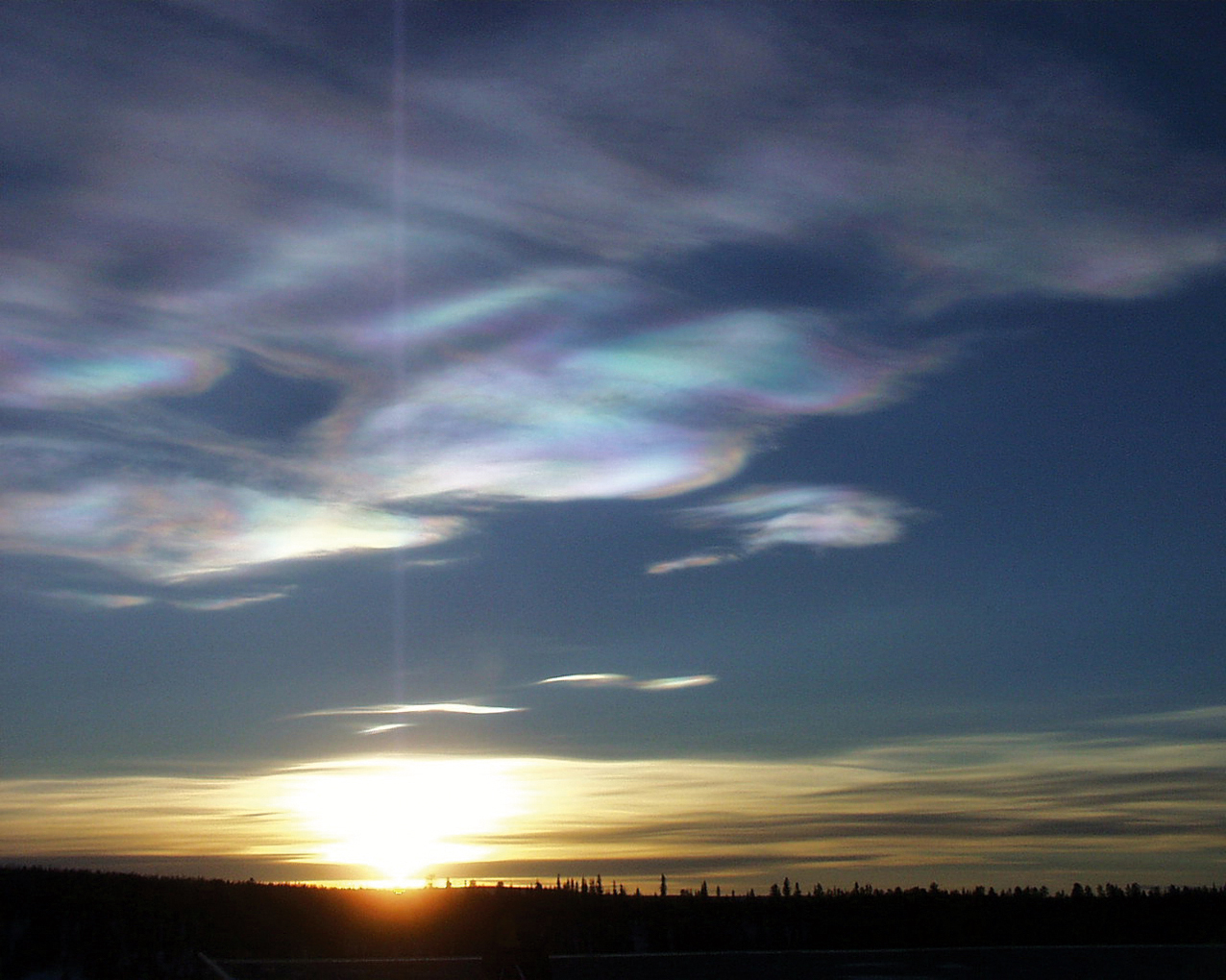
| Fig. 10-18 | Polar
Stratospheric Clouds over Kiruna/Sweden. (photo: H. Berg, Forschungszentrum
Karlsruhe, now with University of Toronto) |
|
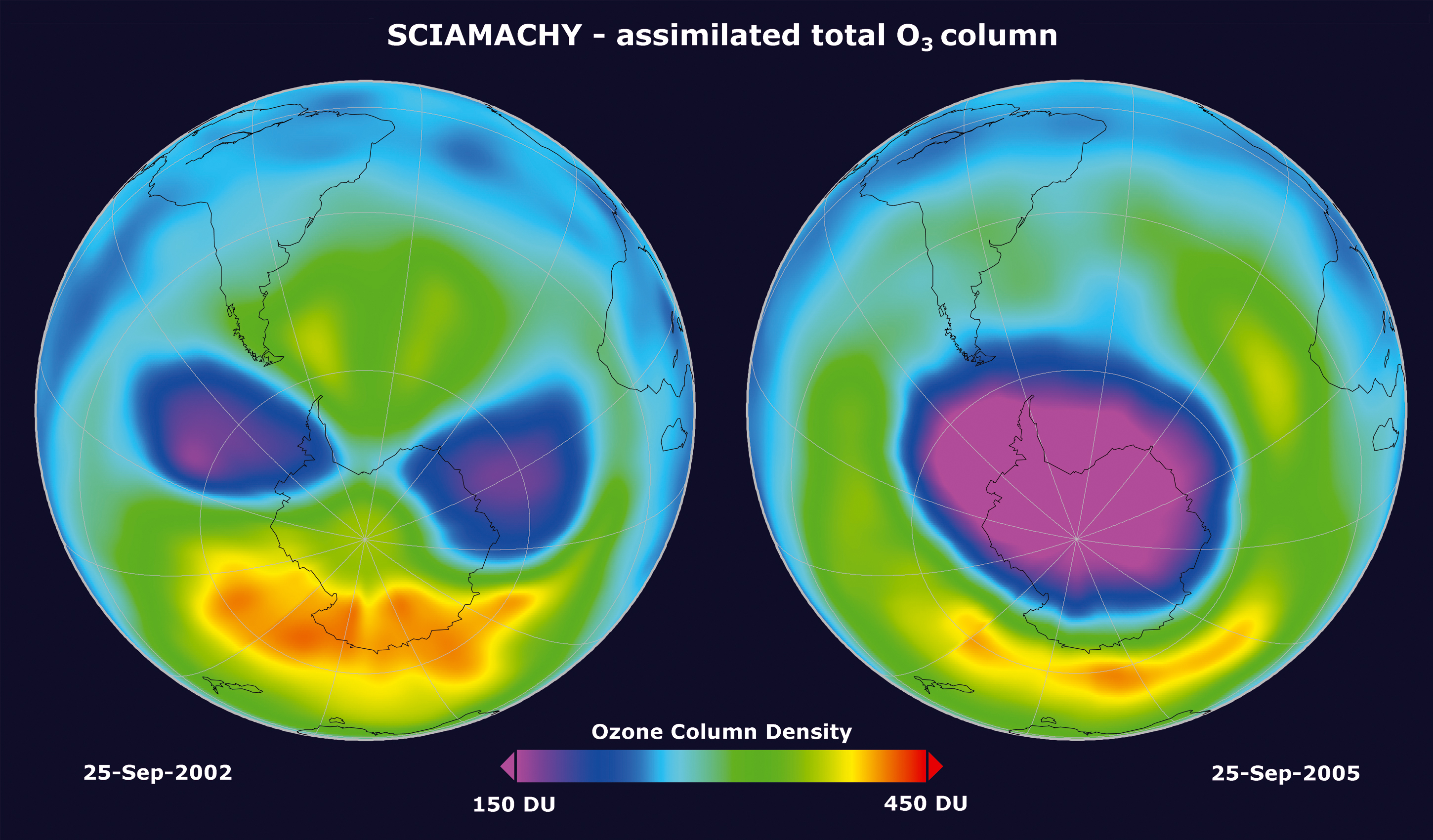
| Fig. 10-19 | The
Antarctic ozone hole in 2002 (left) and 2005 (right). SCIAMACHY total
column ozone measurements from September 25th have been analysed with the ROSE assimilation model to
generate this view. Due to meteorological conditions the hole was split and reduced in size in 2002 but appeared 'as
normal' in 2005. (images: T. Erbertseder, DLR-DFD) |
|
| Fig. 10-20 | Slices
of the polar southern hemisphere ozone field at altitudes of approximately
20, 24 and 28 km on September 27th, 2002 and September 27th, 2005 as measured by SCIAMACHY. The observed
split of the ozone hole in 2002 is not so obvious in the lower stratosphere around 20 km, but clearly visible
at 24 and 28 km. In 2005 an ozone hole of 'normal shape' existed at all altitudes. (images: C. von Savigny, IUP-IFE,
University of Bremen) |

|
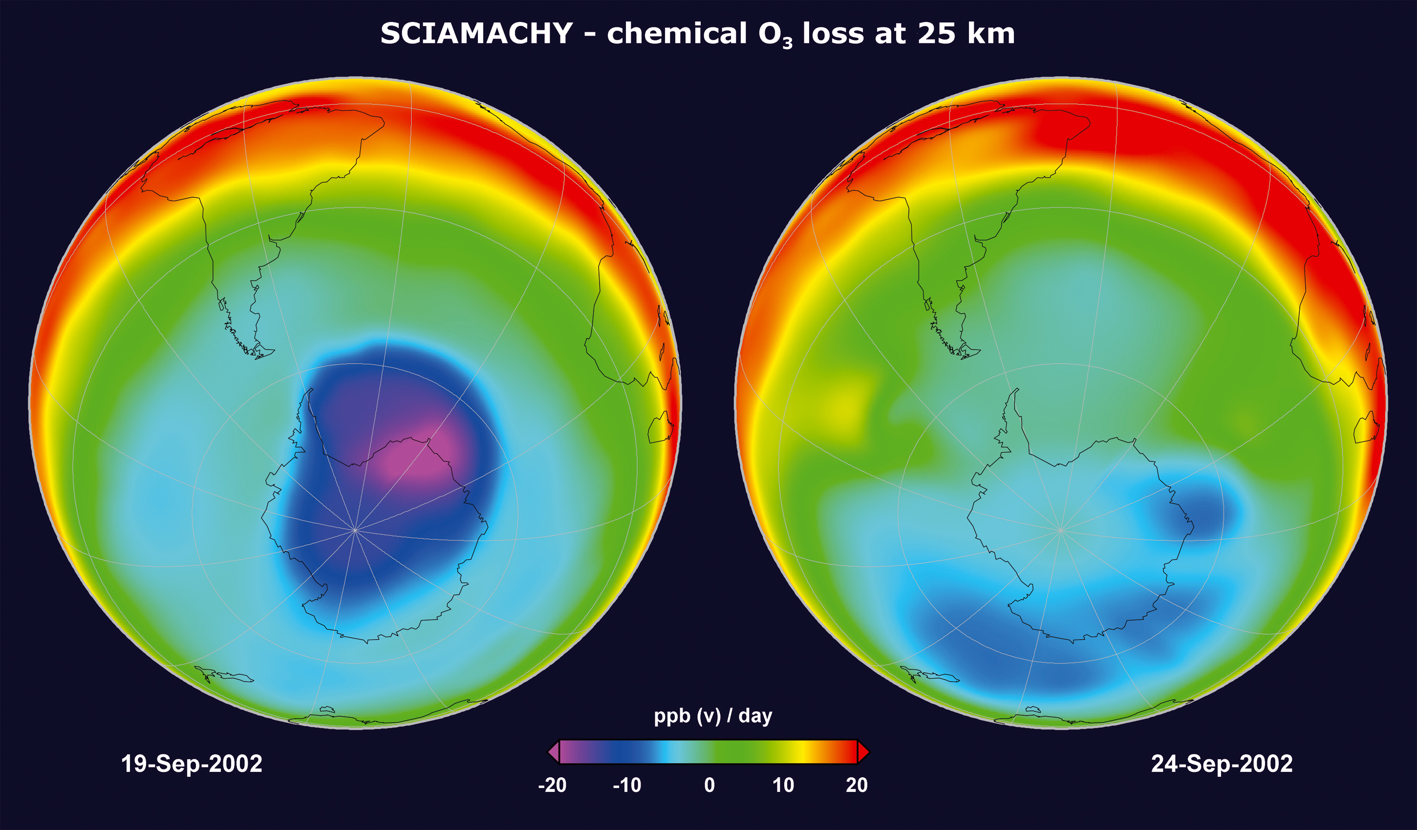
| Fig. 10-21 | Ozone
losses on two days in September 2002 in the mid stratosphere at about
25 km, relative to the previous day. While on September 19th the ozone hole was still developing exhibiting
its usual shape, 5 days later the split-up of the vortex has reduced ozone loss rates as compared to before. (images:
T. Erbertseder, DFD-KA) |
|
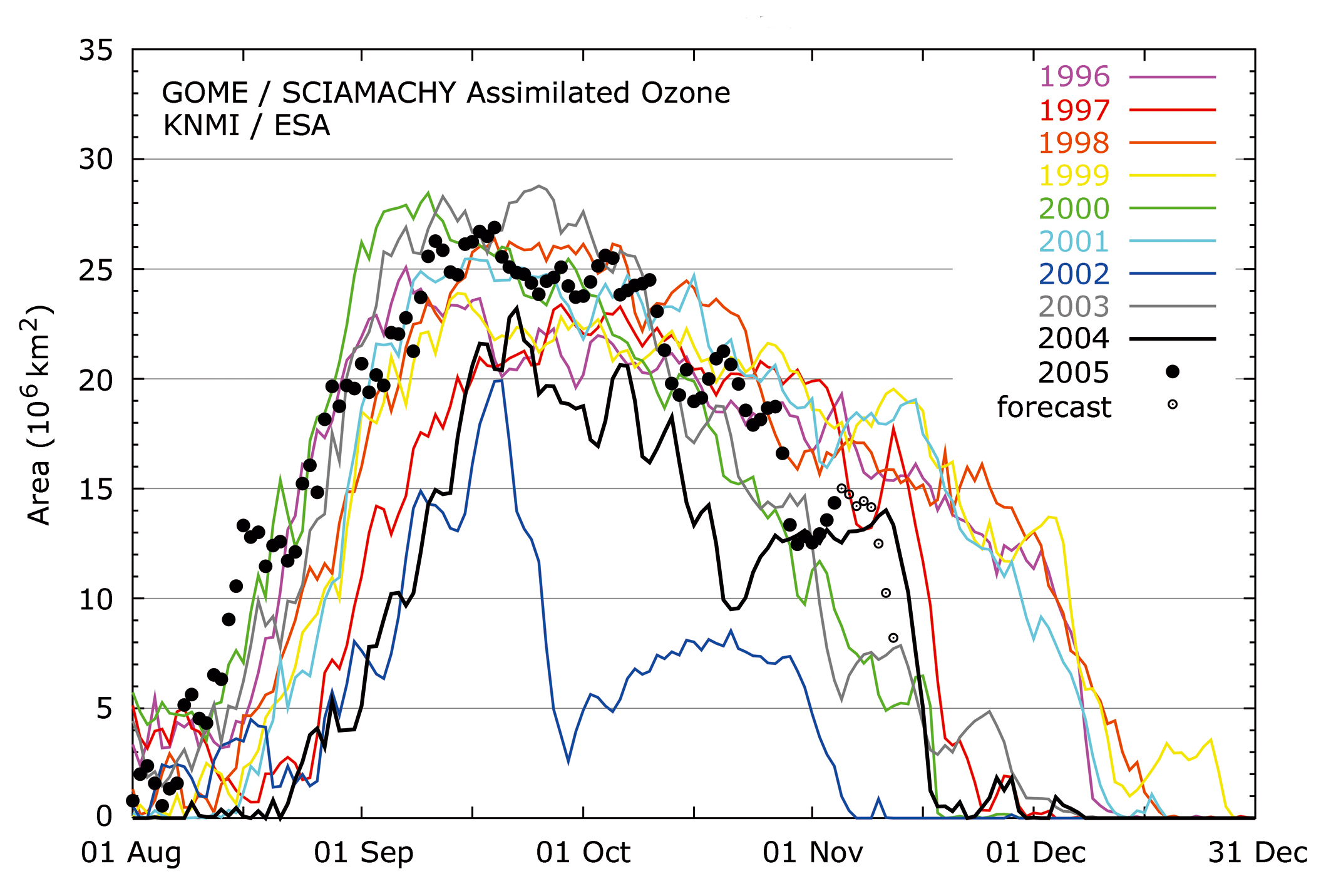
| Fig. 10-22 | Time
series of the size of the Antarctic ozone hole from 1996-2005 based
on observations of GOME and SCIAMACHY. The area includes ozone column values below 30° south lower than
220 Dobson Units. (graphics: KNMI/ESA) |
|
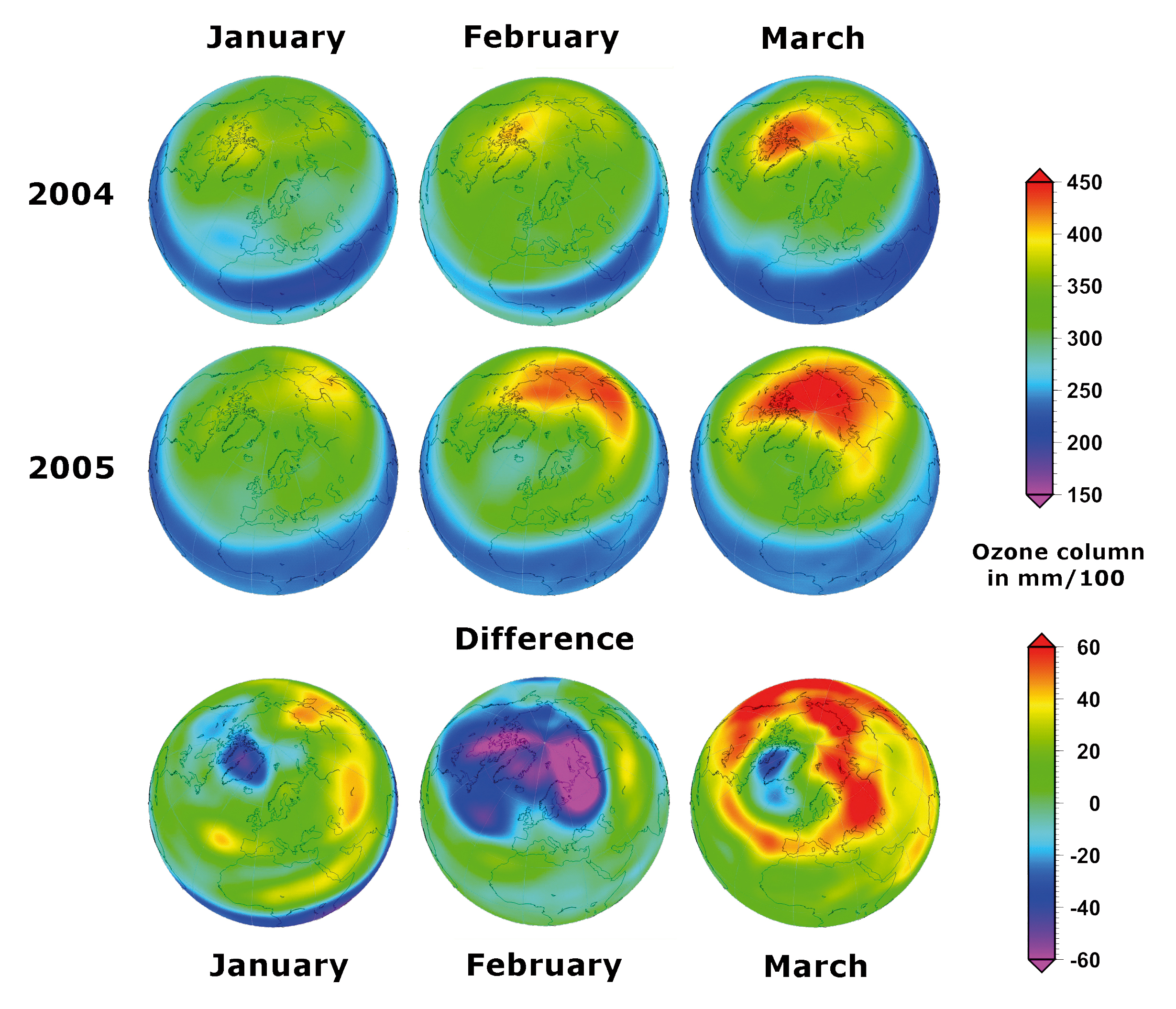
| Fig. 10-23 | Ozone
columns over the northern hemisphere for late winter/early spring 2005
(mid row), 2004 (top row) and the difference between both years (bottom row). Caused by unusual low temperatures
in the stratosphere over the Arctic, significant ozone loss occurred in February 2005 with a recovery of the ozone layer
in March. (images: J. Meyer-Arnek, DLR-DFD) |
|
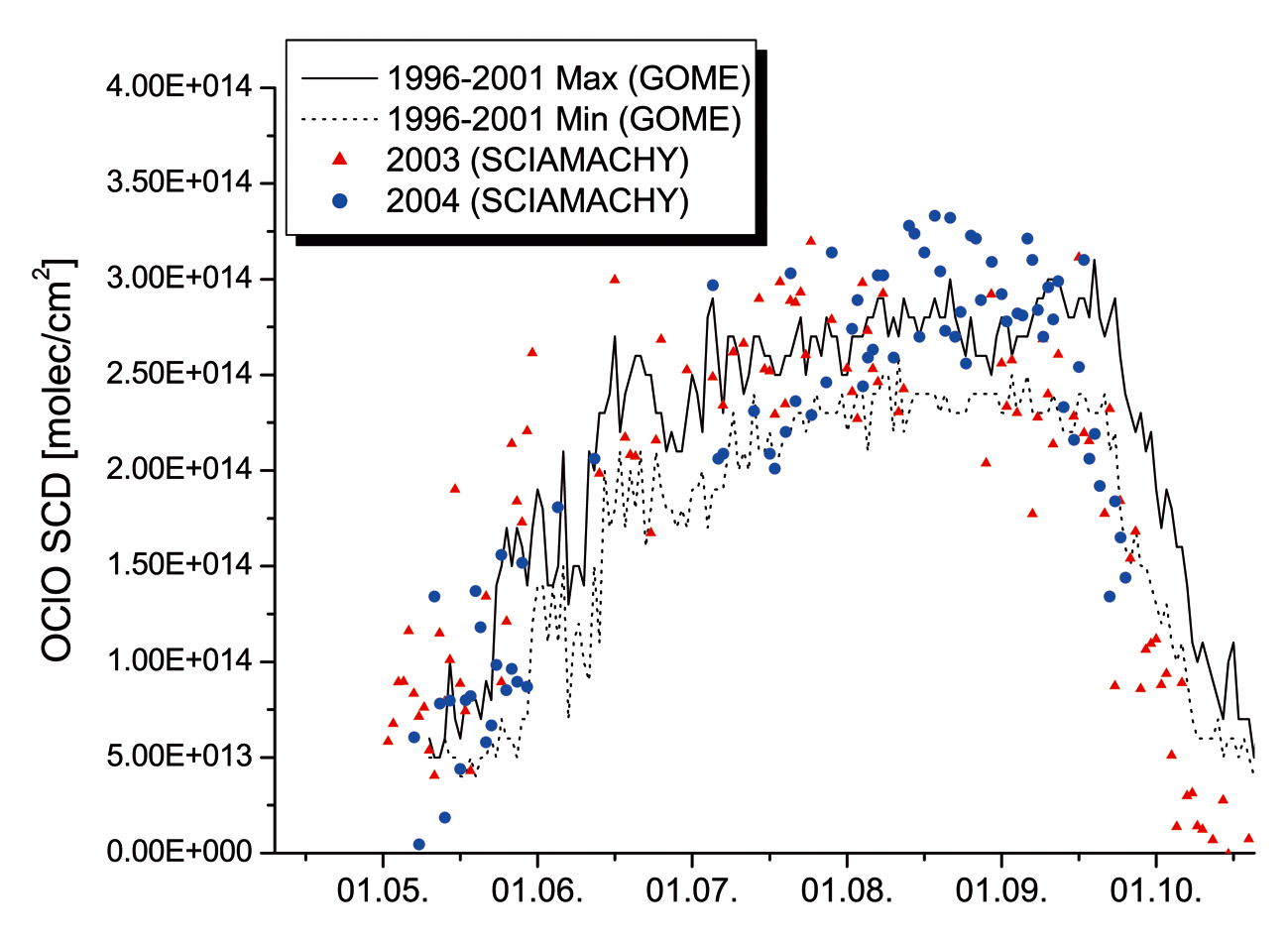
| Fig. 10-24 | OClO
densities in the stratosphere of the southern hemisphere since 1996. SCIAMACHY retrievals fit
well to the GOME time series. High OClO values coincide with the ozone hole season. (graphics: Kühl et al. 2006) |
|
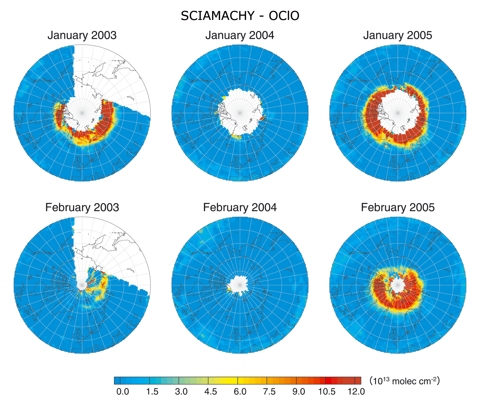
| Fig. 10-25 | Chemically
active chlorine concentrations in the northern hemisphere in winter
2003-2005. Mild winters produce small, very cold winters – like 2005 – very large amounts
of chlorine as depicted by the red areas in the 2005 OCIO maps. (images: A. Richter, IUP-IFE, University of Bremen) |
|
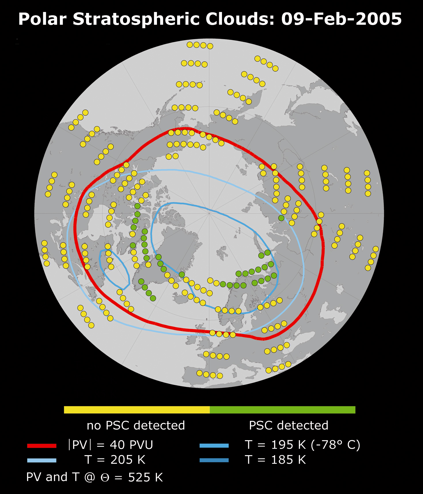
| Fig. 10-26 | Northern
hemisphere map of PSCs for February 9th, 2005. The circles indicate the locations of
limb measurements with green circles corresponding to detected PSCs. They are
superimposed to the UK MetOffice temperature field at 525 K potential temperature, i.e. an altitude of about
22 km, and agree well with the temperature threshold for their formation. The temperature
of 185 K was not reached on February 9th, 2005. (image: C. von Savigny/K.U. Eichmann IUP-IFE, University of Bremen) |
|
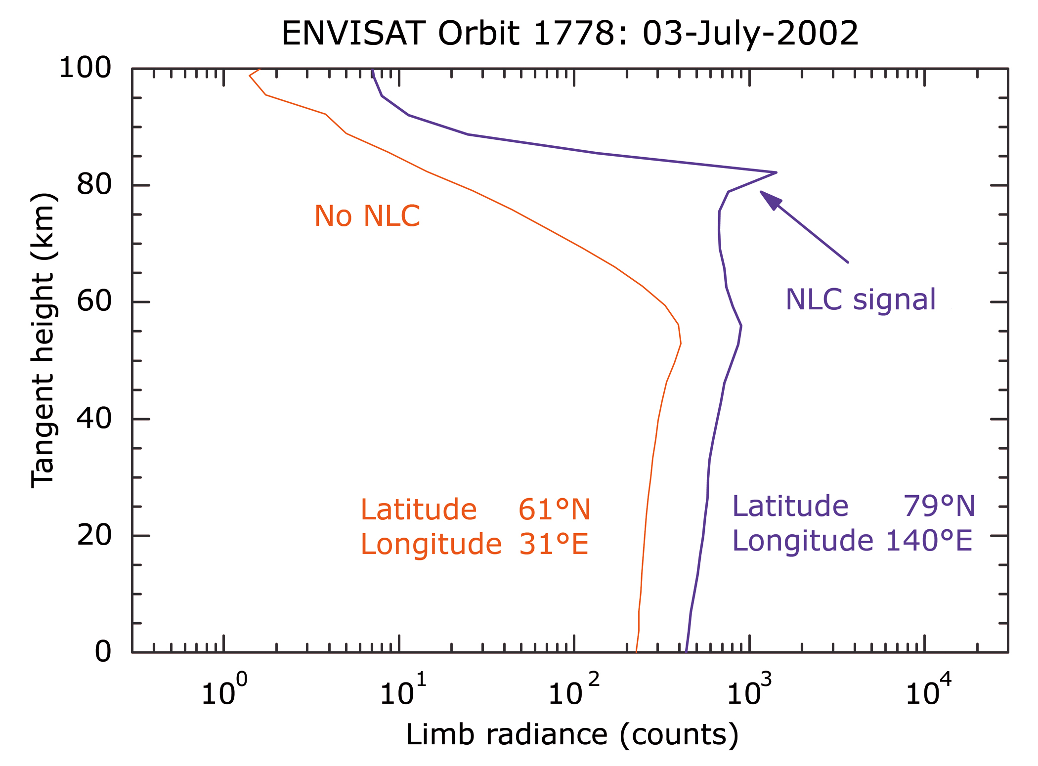
| Fig. 10-27 | NLC
signature in UV limb radiance profiles. The scattering by ice particels in the NLC
leads to a significant increase of the observed limb radiance profiles peaking at the characteristic
NLC altitude of about 83-85 km (blue line). Shown in red is for comparison a limb radiance
measurement without NLCs being present. (graphics: C. von Savigny, IUP-IFE, University of Bremen) |
|
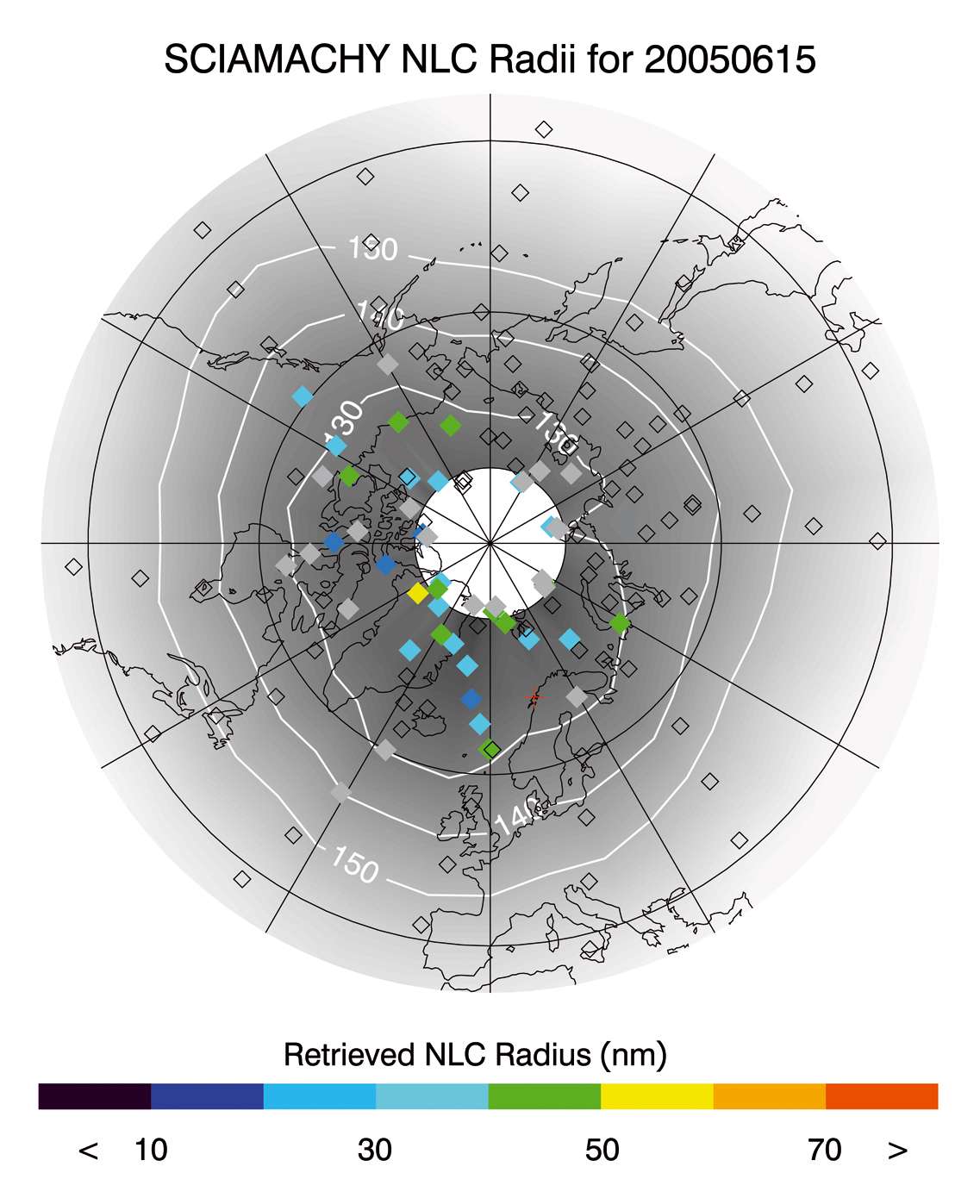
| Fig. 10-28 | NLC
particle sizes for June 15th, 2005 derived from SCIAMACHY limb measurements. The grey solid diamonds
indicate thin – but detectable – NLCs that did not allow a reliable size determination. The white
contours indicate the temperature field at 83 km altitude as measured with AURA/MLS. (image: C. von Savigny, IUP-IFE,
University of Bremen) |
|
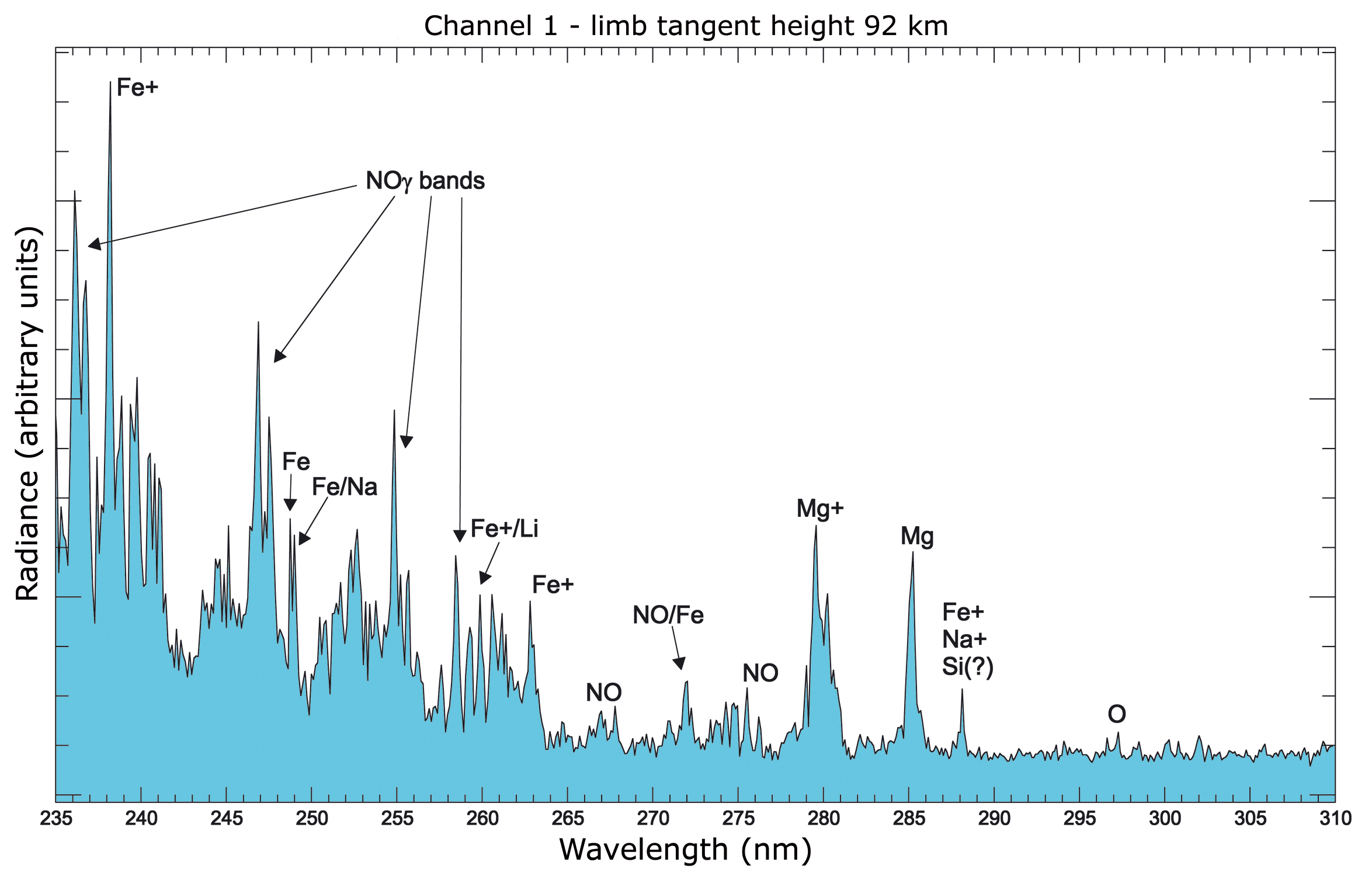
| Fig. 10-29 | Emission
lines in SCIAMACHY limb radiance in channel 1 at the highest tangent altitude of about 92 km, normalised
to the solar irradiance, in arbitrary units. A number of emission signals is detected here; the most dominant features
are the NO gamma-bands and MgII, but signals from neutral Mg, atomic oxygen, Si, Fe and Fe+ are observed as well.
(graphics: M. Scharringhausen, IUP-IFE, University of Bremen) |
|
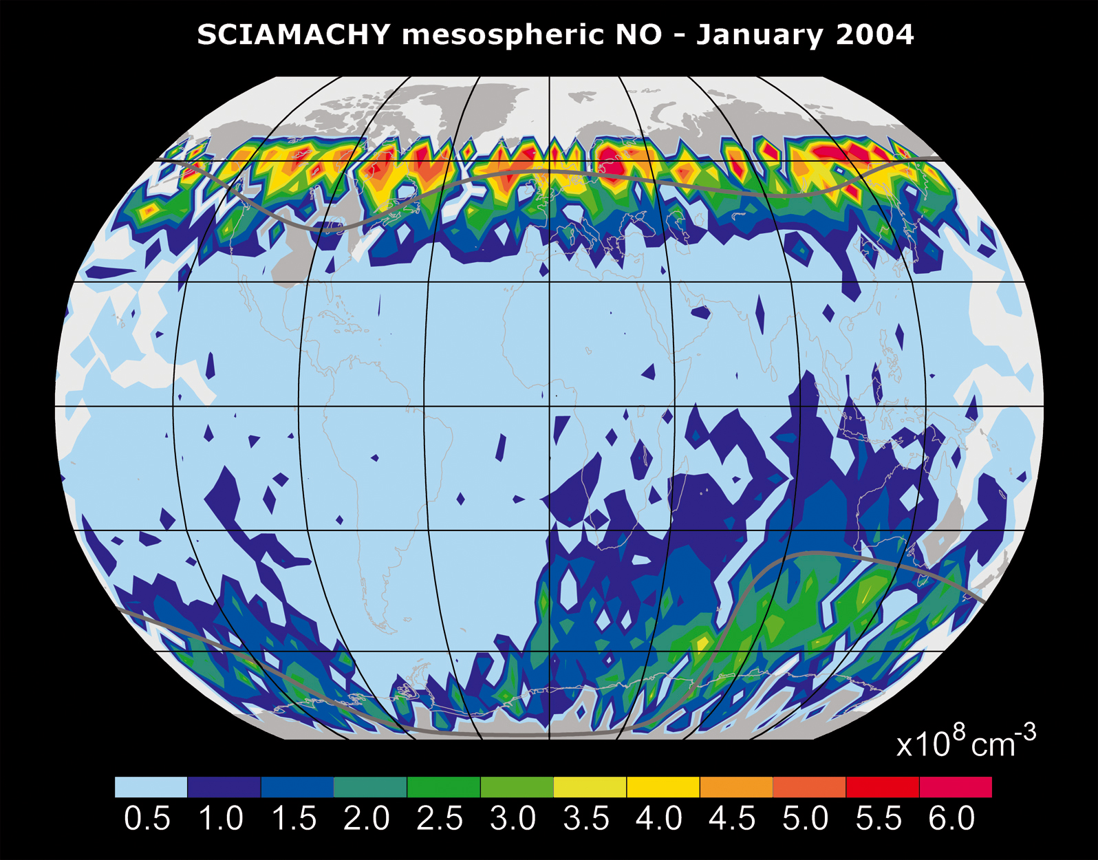
| Fig. 10-30 | Global
distribution of NO number densities at 92 km altitude, averaged over
a 5° grid, monthly average of January 2004. The dark grey lines denote 55° of geomagnetic latitude, i.e.
the outer edge of the auroral oval. Over South America and the South Atlantic the high particle fluxes in the SAA prevent data
retrieval and cause a data gap. No data are available north of 65°, as this area is in polar night. (image: M. Sinnhuber/M.
Scharringhausen, IUP-IFE, University of Bremen) |
|
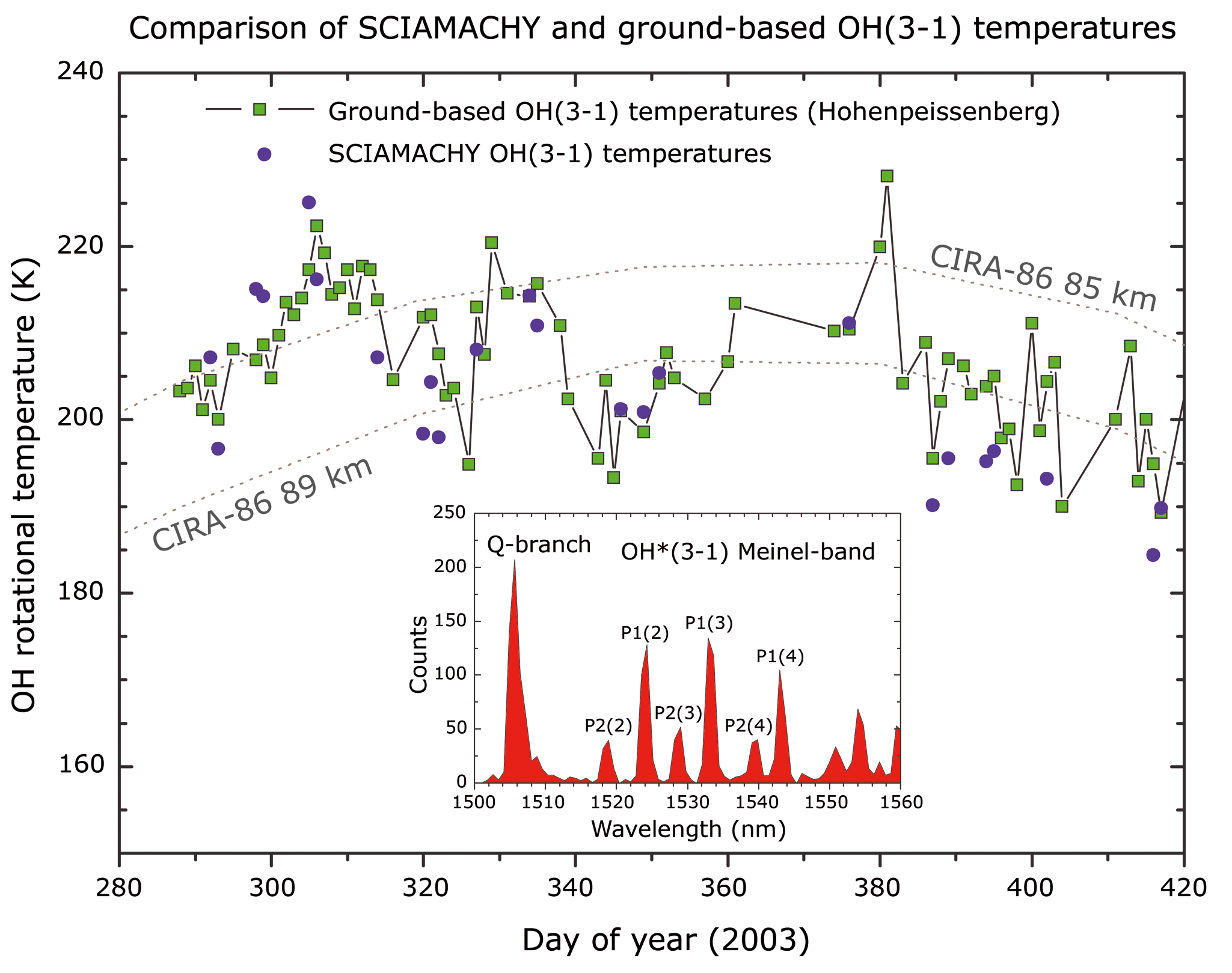
| Fig. 10-31 | Variation
of the temperature at the mesopause derived from SCIAMACHY nighttime limb emission spectra (inset)
in the OH-Meinel bands at a tangent height of 85.5 km. The inset shows the Q-branch (at 1507 nm) and the P-branch rotational
lines of the OH* (3-1) vibrational transition. (image: C. von Savigny, IUP-IFE, University of Bremen with ground based
measurements kindly provided by M. Bittner and D. Offermann) |
|
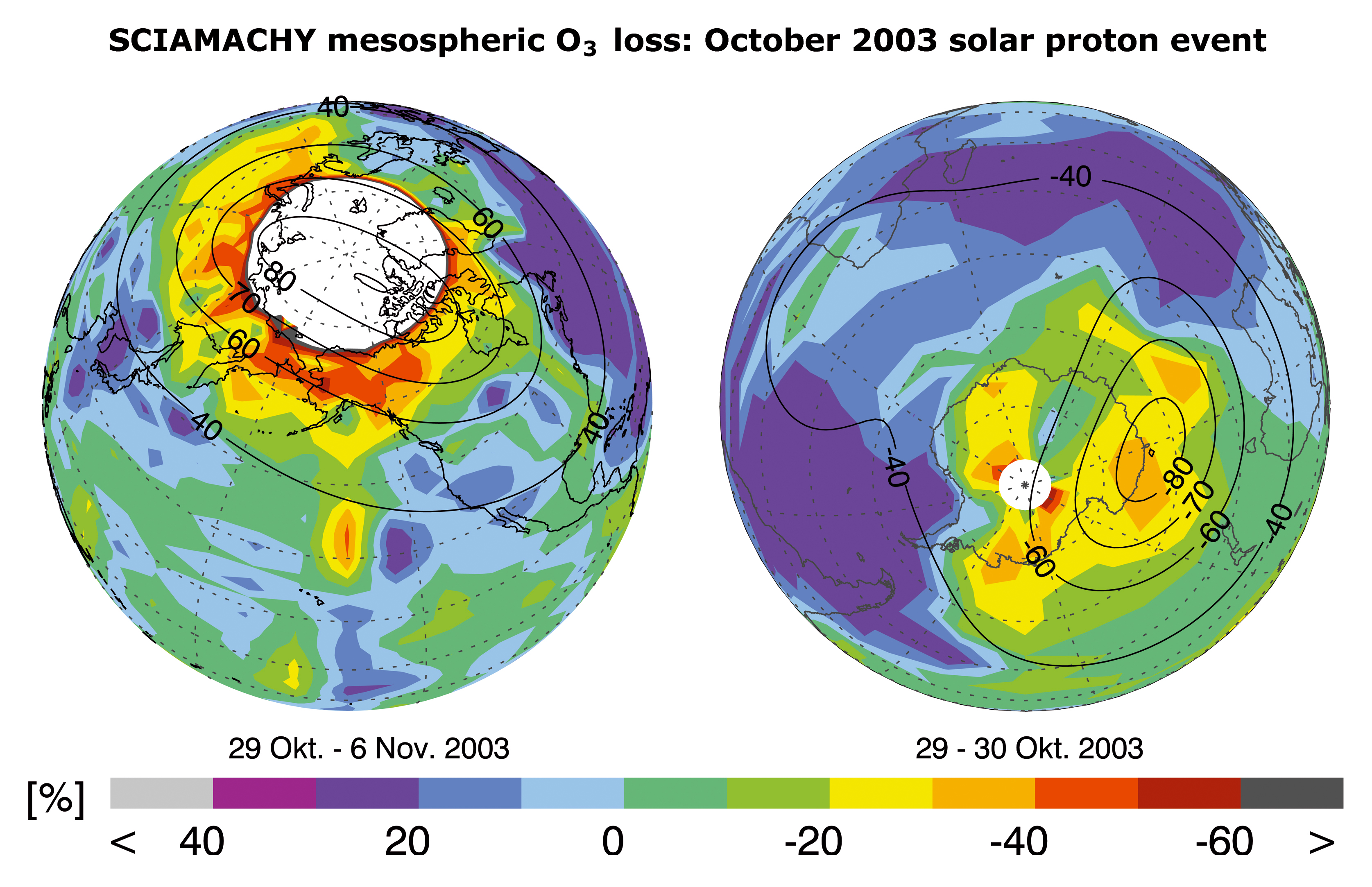
| Fig. 10-32 | Measured
change of ozone concentration at 49 km altitude due to the strong solar
proton events end of October 2003 in the northern and southern hemisphere relative to the reference
period of October 20-24, 2003. White areas depict regions with no observations. The black solid lines are the Earth’s
magnetic latitudes at 60 km altitude for 2003. (image: Rohen et al. 2005) |
|
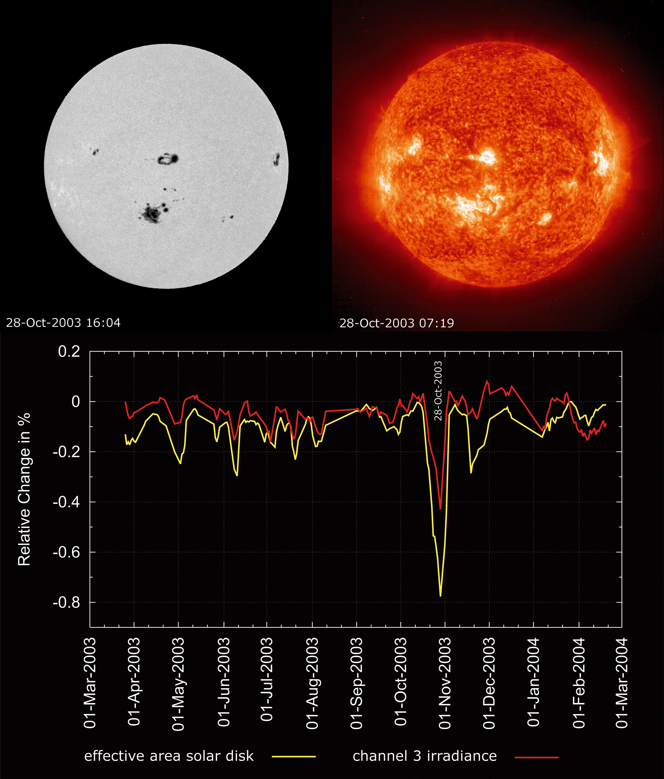
| Fig. 10-33 | The
active sun on October 28th, 2003, in white light (top left), EUV at 304 Å (top right) and the signal in
channel 3 as measured by SCIAMACHY. (images: Big Bear Solar Observatory, SOHO and IUP-IFE, University of Bremen) |
|
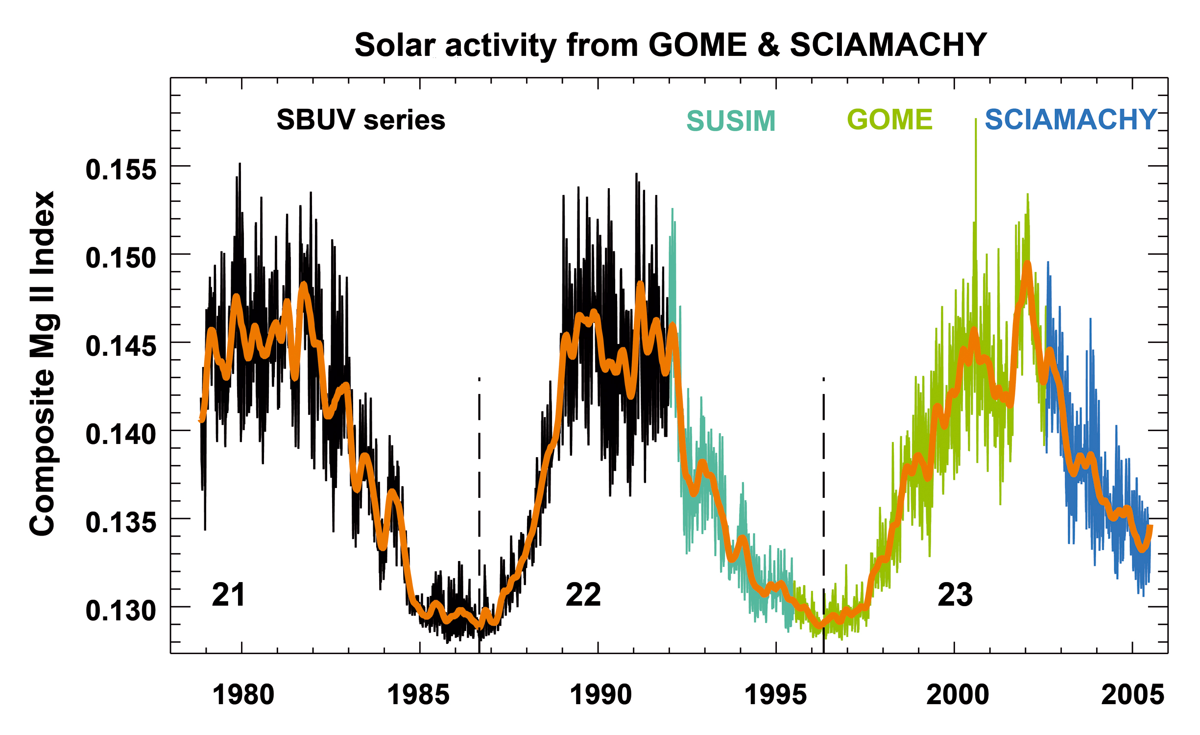
| Fig. 10-34 | Solar
activity measured via the Mg II index by several satellite instruments including GOME and SCIAMACHY.
By combining various satellite instruments, the composite Mg II index covers nearly three complete 11-year solar cycles.
(graphics: M. Weber, IUP-IFE, University of Bremen) |
|
| Fig. 10-35 | The
global UV index on November 8th, 2005. Red denotes high, blue low UV irradiance. (image: KNMI/ESA) |

|
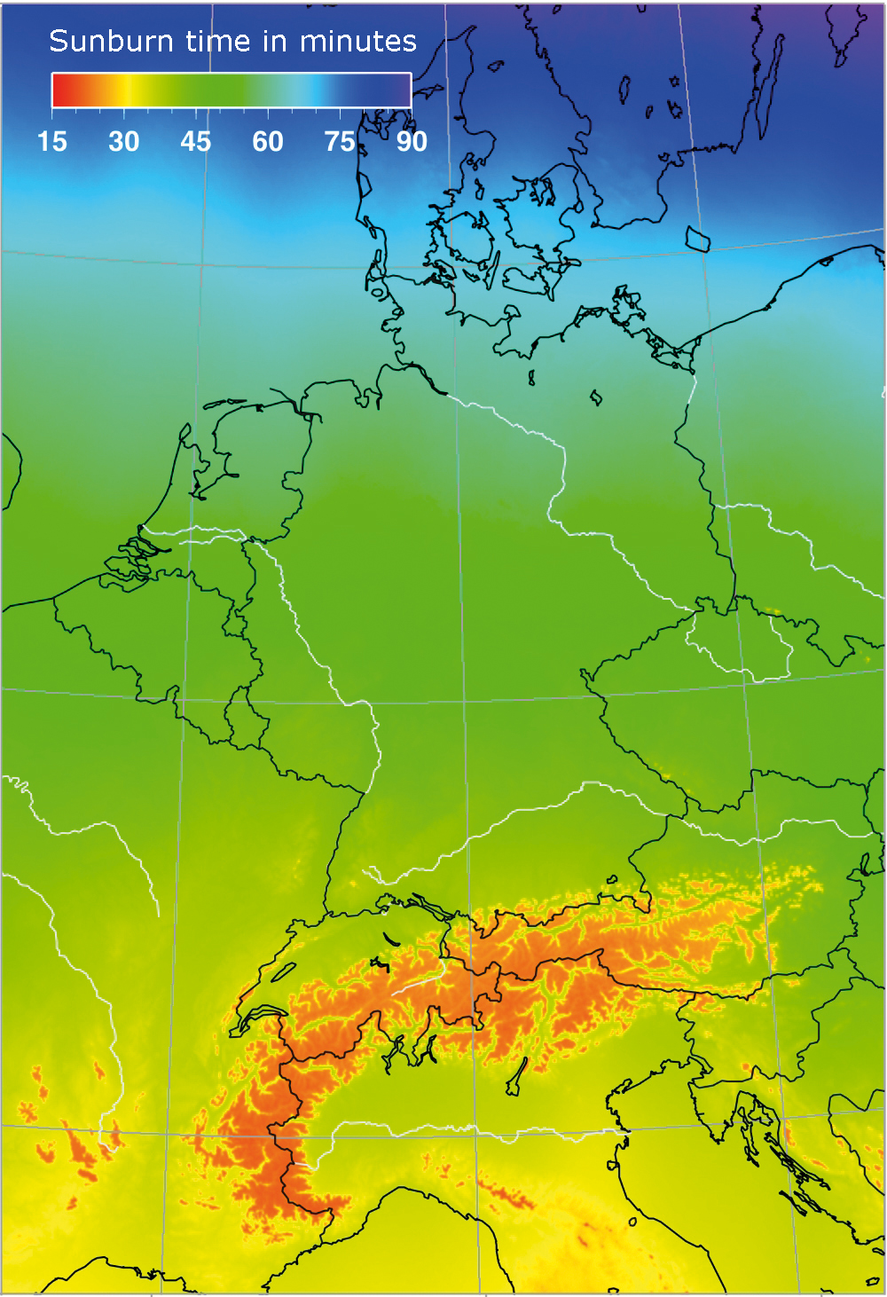
| Fig. 10-36 | The
sunburn time in central Europe in winter. In the Alps at high elevation UV radiation begins to redden
skin after only 20 minutes. (image: T. Erbertseder, DLRDFD) |
|
Page generated 26 March 2007