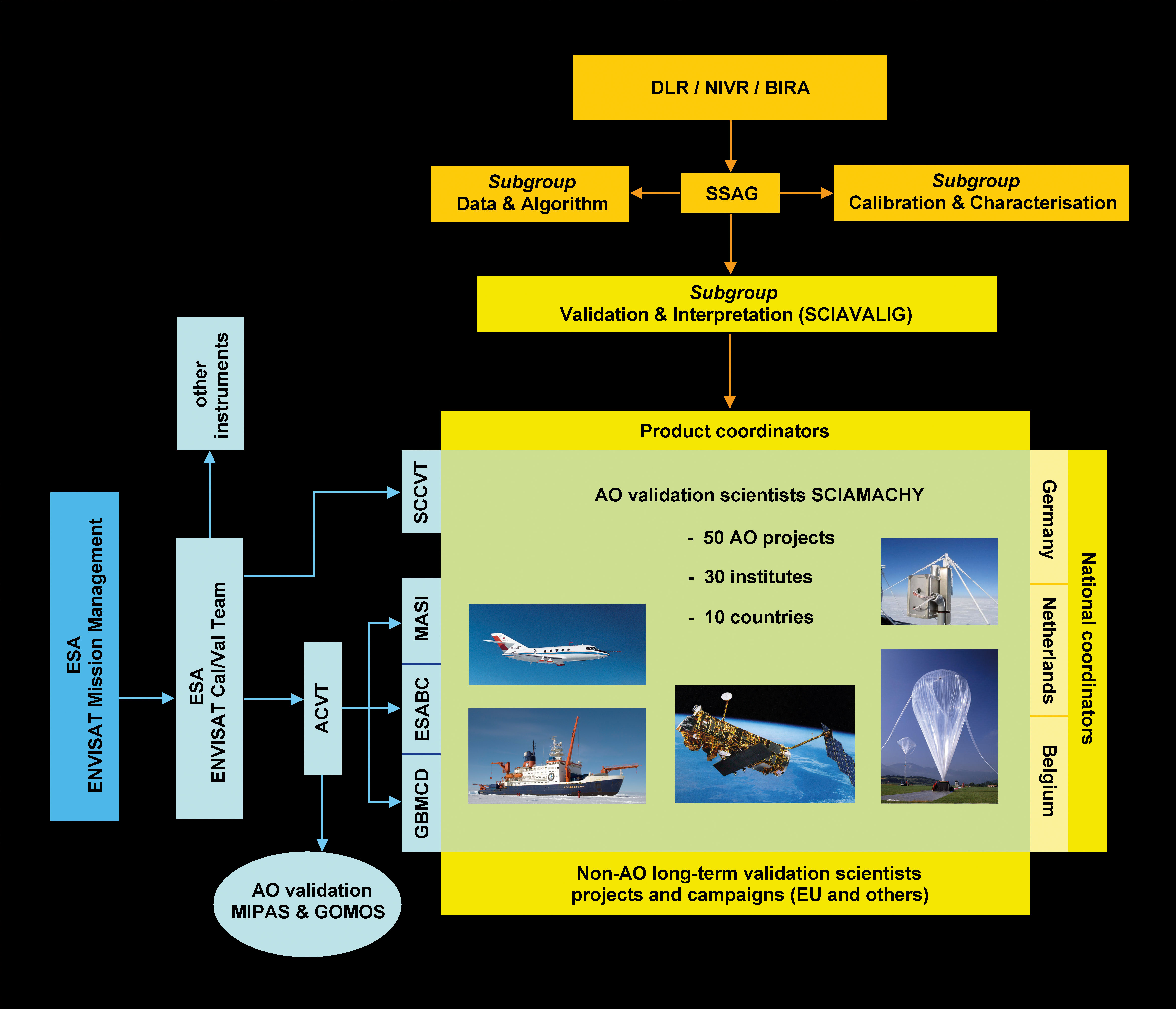
| Fig. 9-1 |
A scheme of the SCIAMACHY validation organisational structures setup by
SCIAVALIG (light orange) and by ESA (pale blue). The validation scientists actually doing the work are supported by
both organisations, if they have an approved AO proposal for SCIAMACHY validation (green). (Courtesy: KNMI/DLR-IMF) |
|
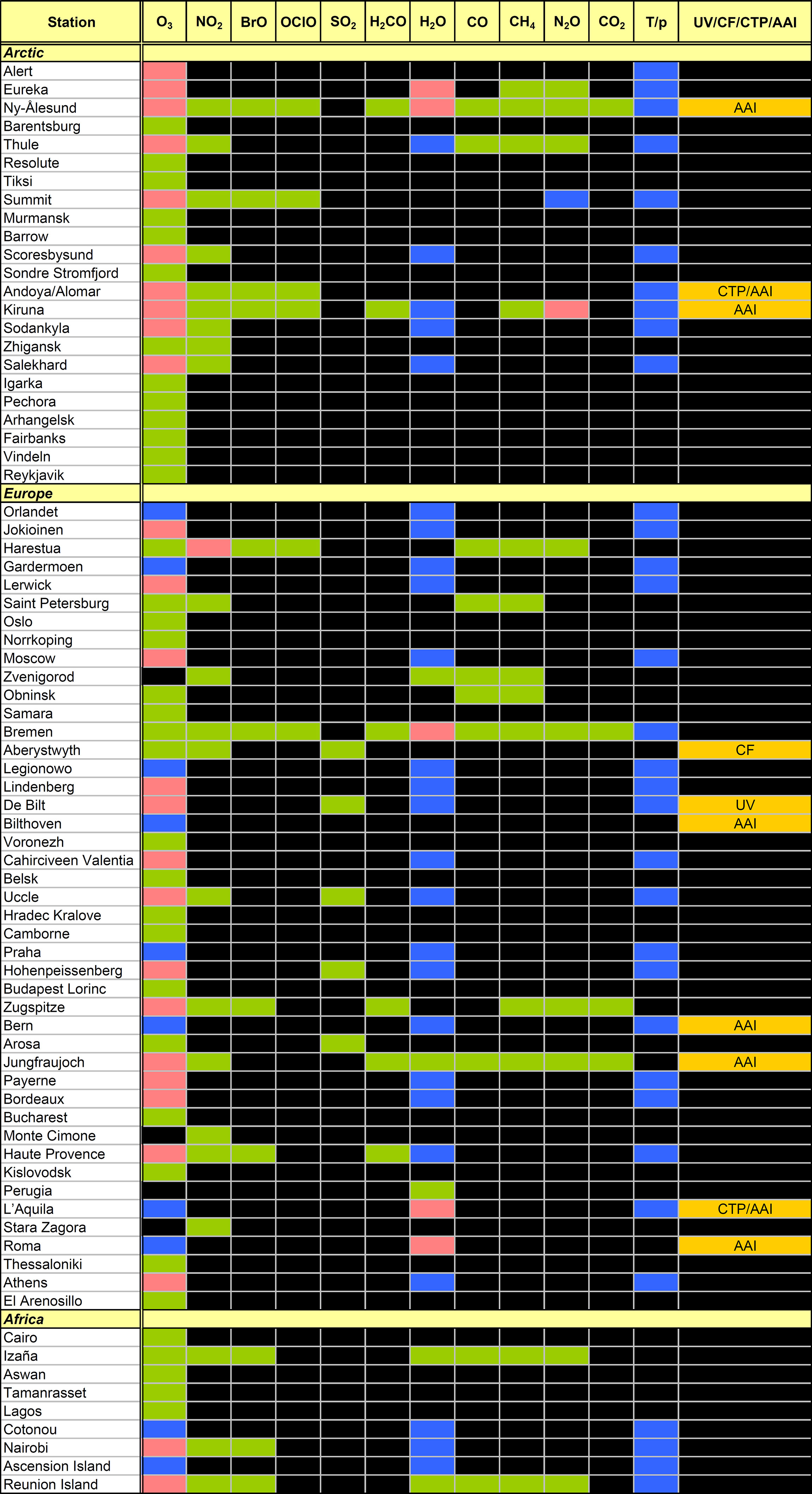
| Fig. 9-2a |
Ground-based stations contributing to SCIAMACHY validation and associated SCIAMACHY data products.
The last column includes UV, CF (cloud fraction), CTP (cloud top pressure) and AAI (absorbing aerosol index).
Courtesy: KNMI/DLR-IMF) |
|
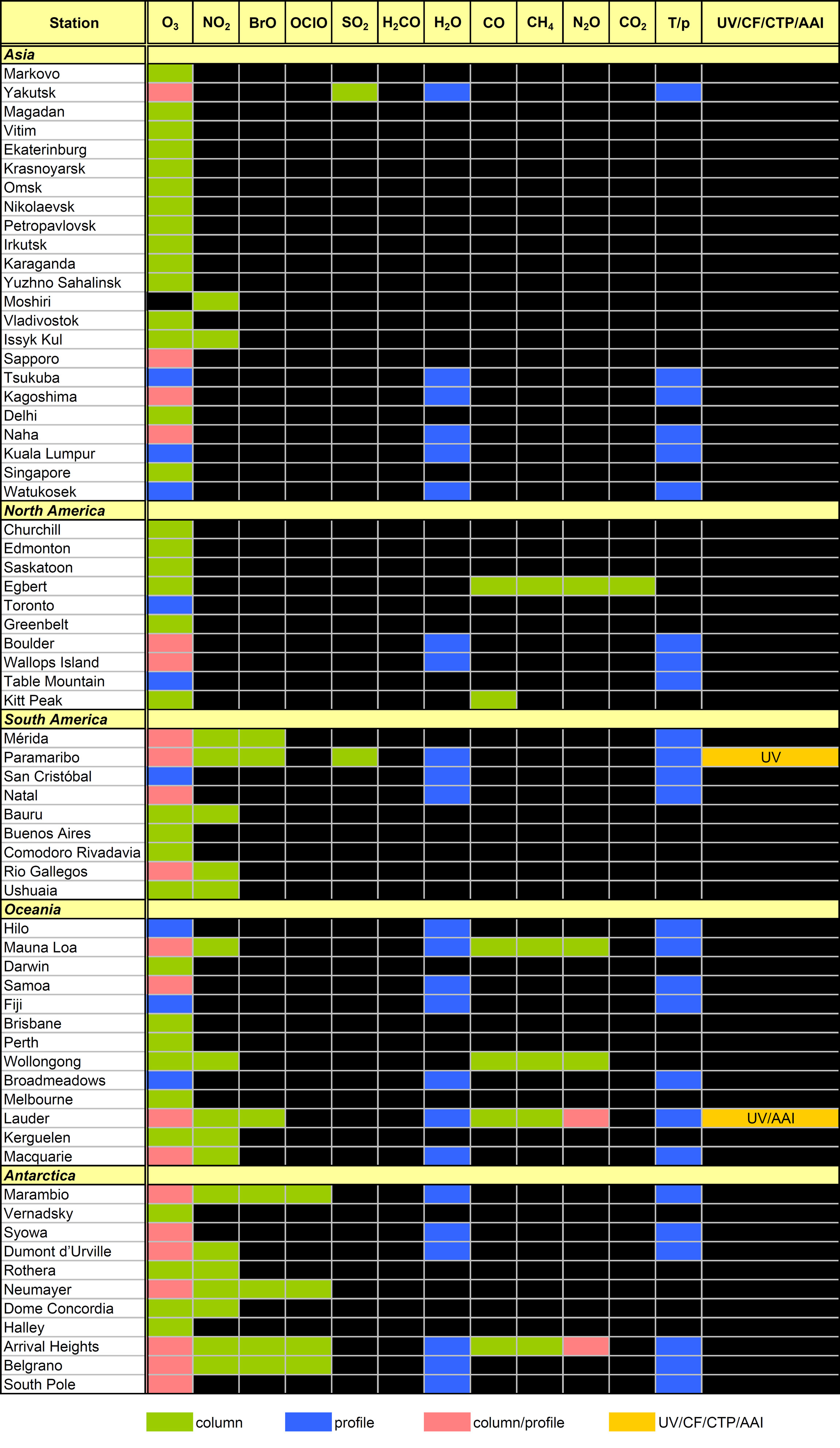
| Fig. 9-2 (continued) |
|
|
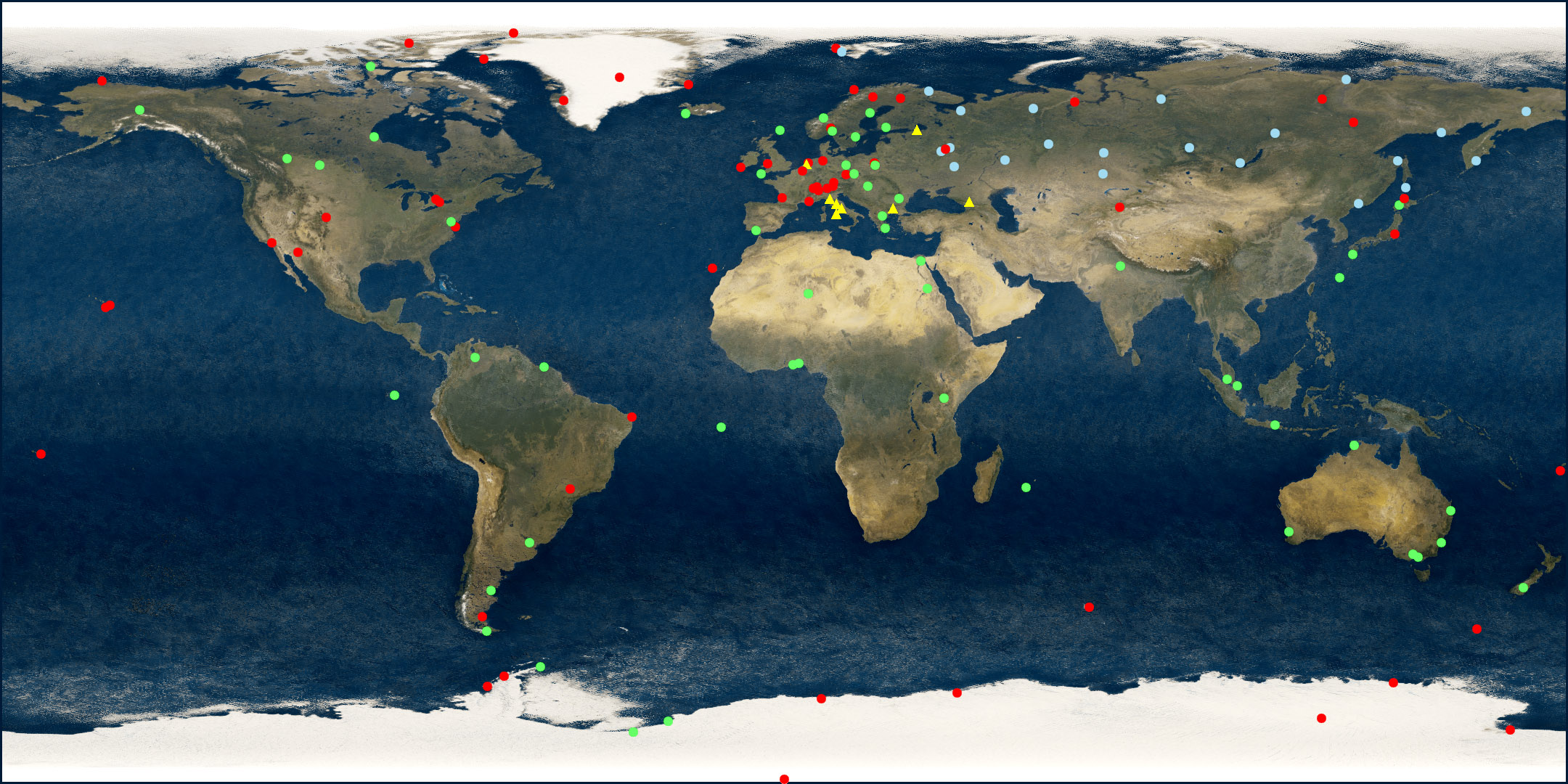
| Fig. 9-3 |
Global distribution of validation sites. Symbols and colour codes indicate the prime network as follows:
red circles = NDACC, blue circles = Russian/NIS M-124, green circles = GAW, yellow triangles = others.
(Courtesy: DLR-IMF/SRON/KNMI) |
|
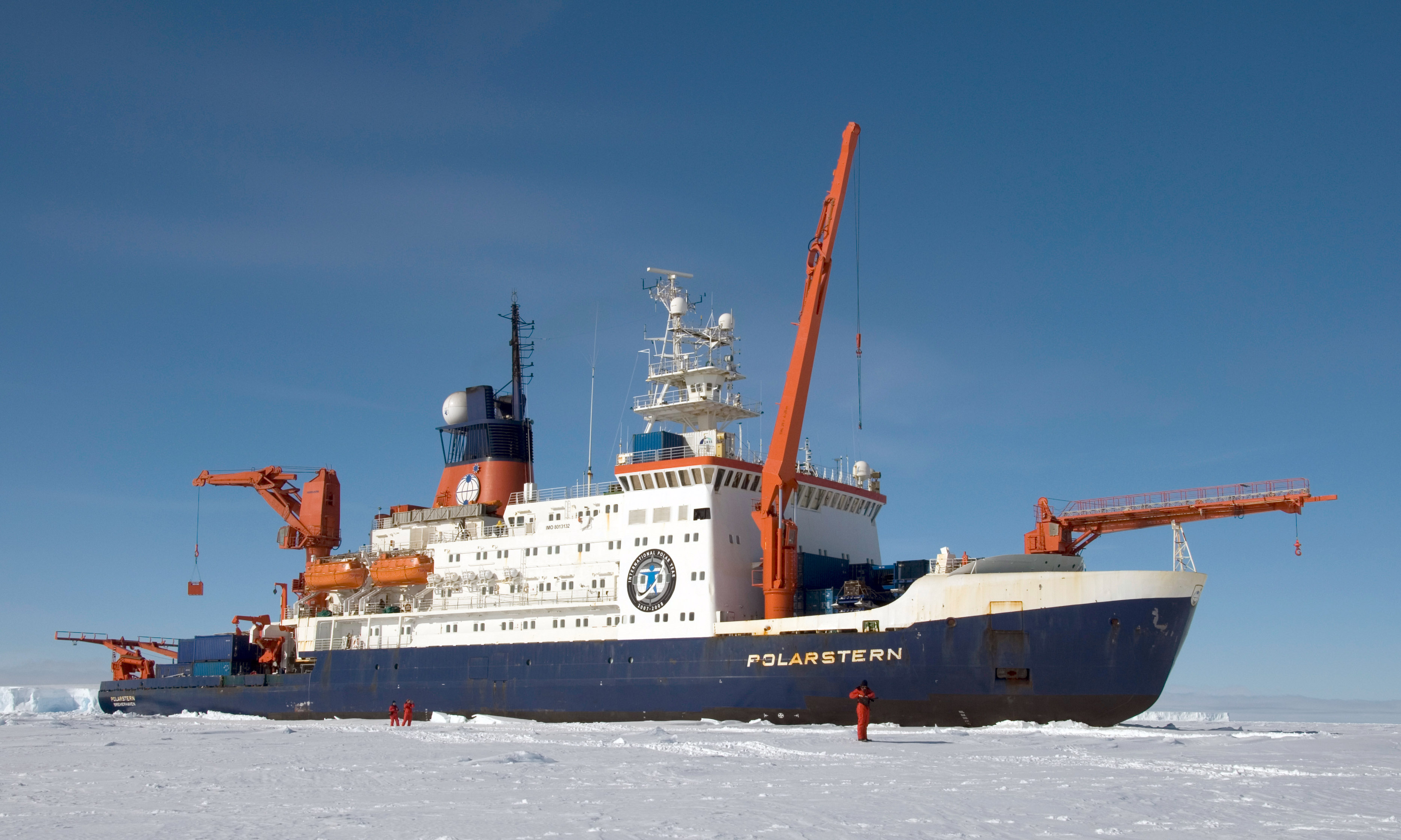
| Fig. 9-4 |
The research vessel Polarstern. (Photo: G. Chapelle/Alfred Wegener Institute for Polar and Marine Research) |
|
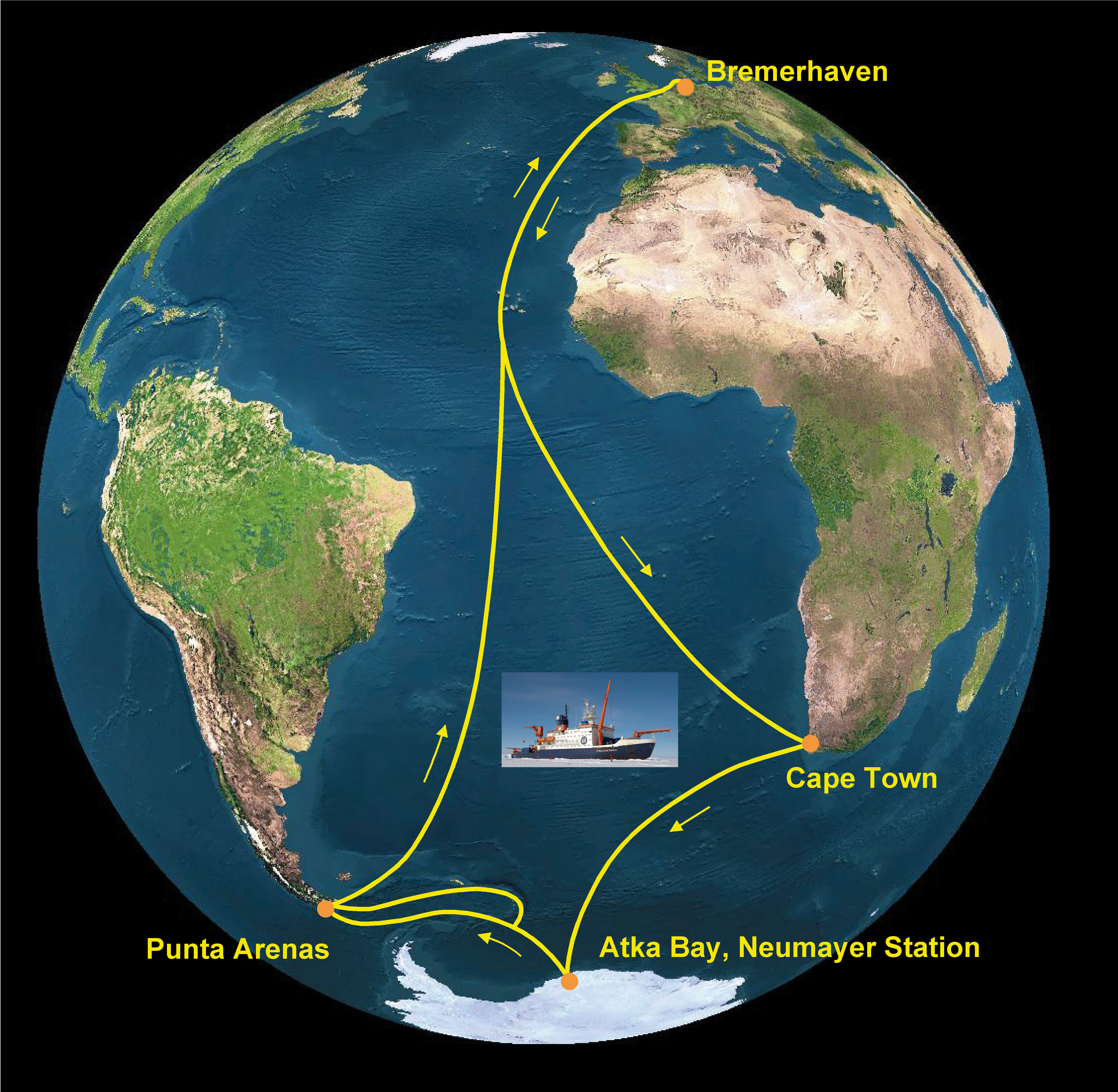
| Fig. 9-5 |
Route of the Polarstern cruise during the ANT XIX campaign between November 2001 and May 2002. (Courtesy: DLR-IMF) |
|
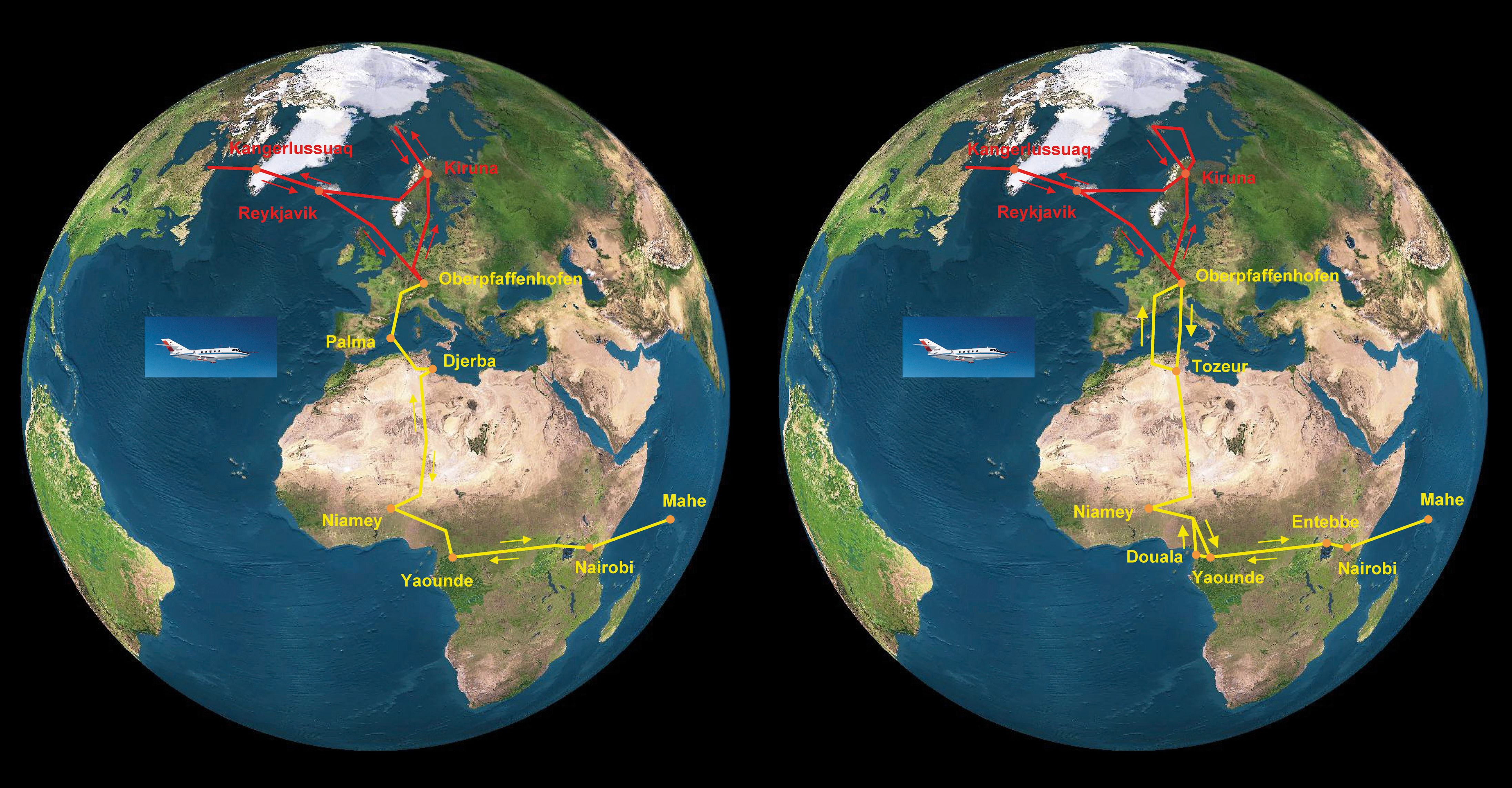
| Fig. 9-6 |
Falcon flight tracks for the September 2002 (left) and February/March 2003 (right) SCIA-VALUE airborne campaigns.
Displayed in red are the northern tracks (3-8 September 2002 and 19 February - 3 March 2003) while the southern tracks
(15-28 September 2002 and 10-19 March 2003) are displayed in yellow. (Courtesy: DLR-IMF) |
 |
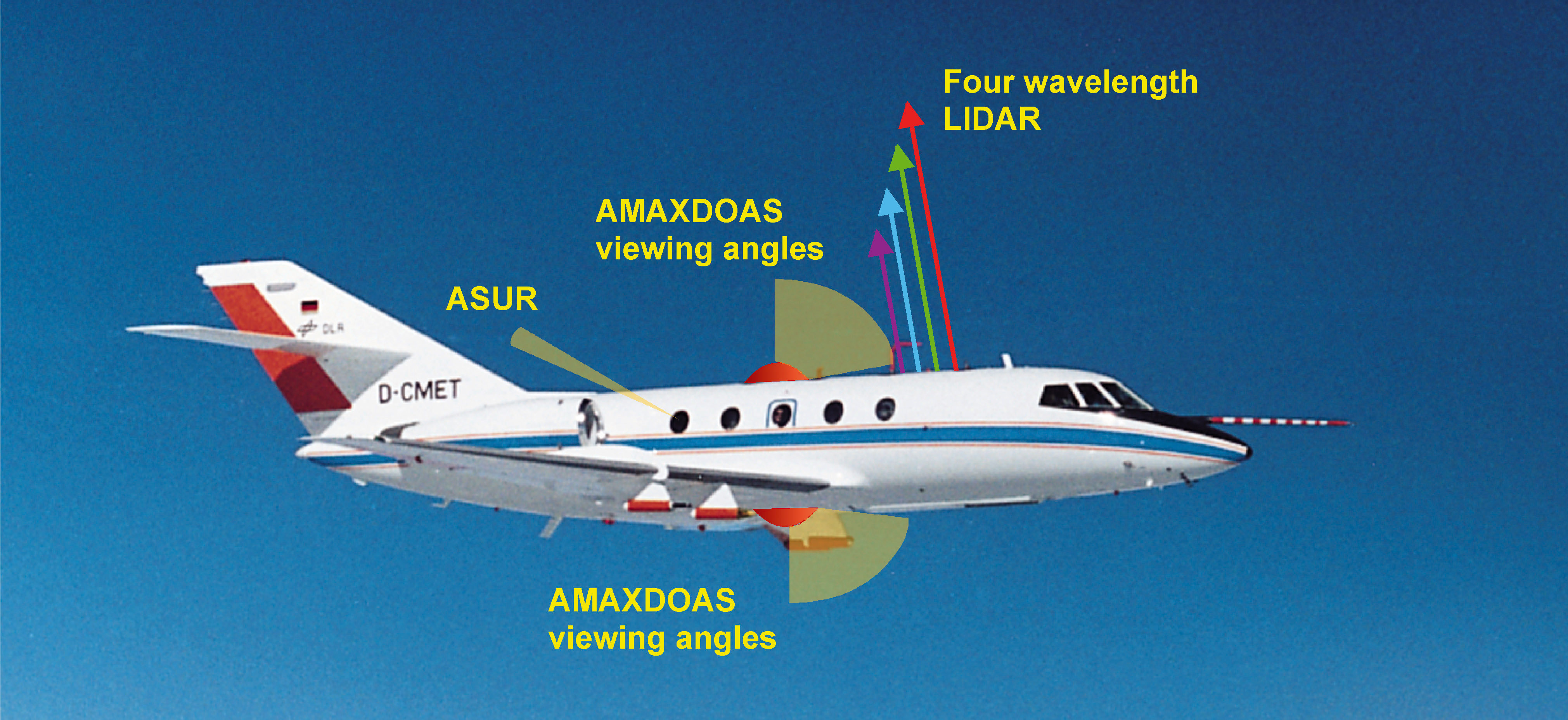
| Fig. 9-7 |
The Falcon aircraft with the viewing directions of the validation instruments. (Courtesy: Fix et al. 2005) |
|
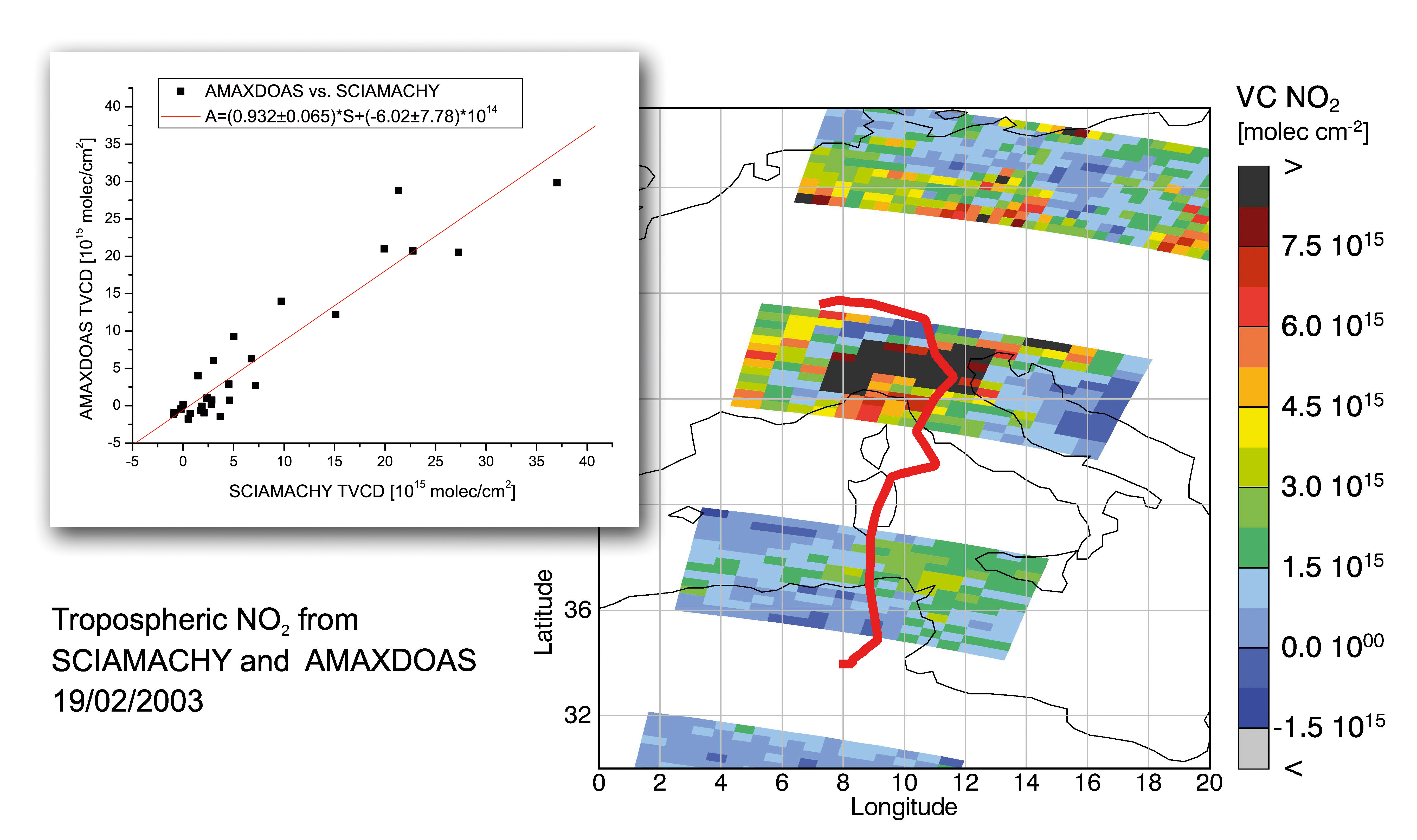
| Fig. 9-8 |
Tropospheric NO2 column obtained by SCIAMACHY together with the Falcon flight track (in red) showing where
AMAX-DOAS measured almost simultaneously. In the inset, tropospheric NO2 columns from AMAX-DOAS are plotted versus
those from SCIAMACHY. The SCIAMACHY tropospheric NO2 columns are retrieved by IUP-IFE, University of Bremen.
(Courtesy: Heue et al. 2005) |
|
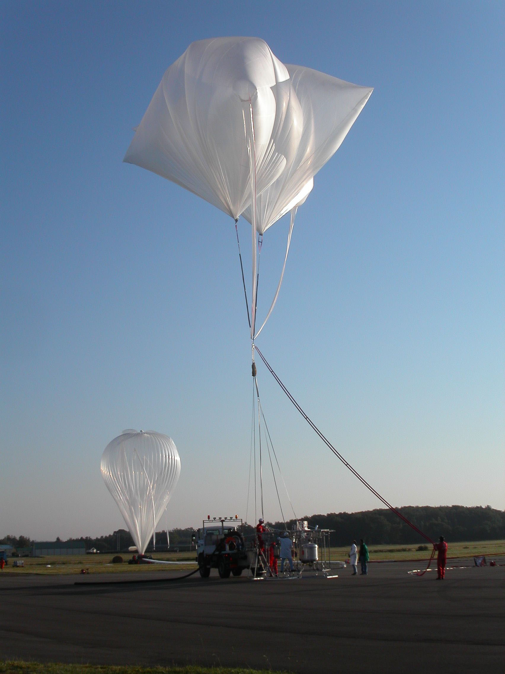
| Fig. 9-9 |
Launch of the TRIPLE payload in Aire sur l'Adour in September 2002. (Photo: W. Gurlit, IUP-IFE, University of Bremen) |
 |
| Fig. 9-10 |
The difference between total O3 columns retrieved from SCIAMACHY and selected ground stations for the years 2002-2008.
The red curve indicates seasonal variability and long-term trends obvious in the comparison. The
trends range between -0.15% and -1.1% per year. (Courtesy: adapted from Lerot et al. 2009) |
 |
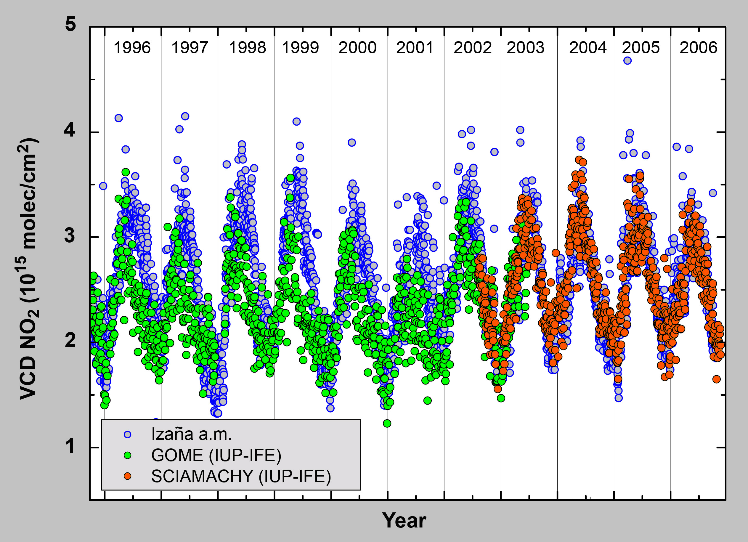
| Fig. 9-11 |
NO2 vertical column densities from SCIAMACHY nadir measurements (red) compared with ground-based morning data from
Izaña (grey) and VCD from GOME (green). The GOME and SCIAMACHY VCD have been retrieved with a scientific algorithm
from IUP-IFE, University of Bremen. (Courtesy: Gil et al. 2008) |
|
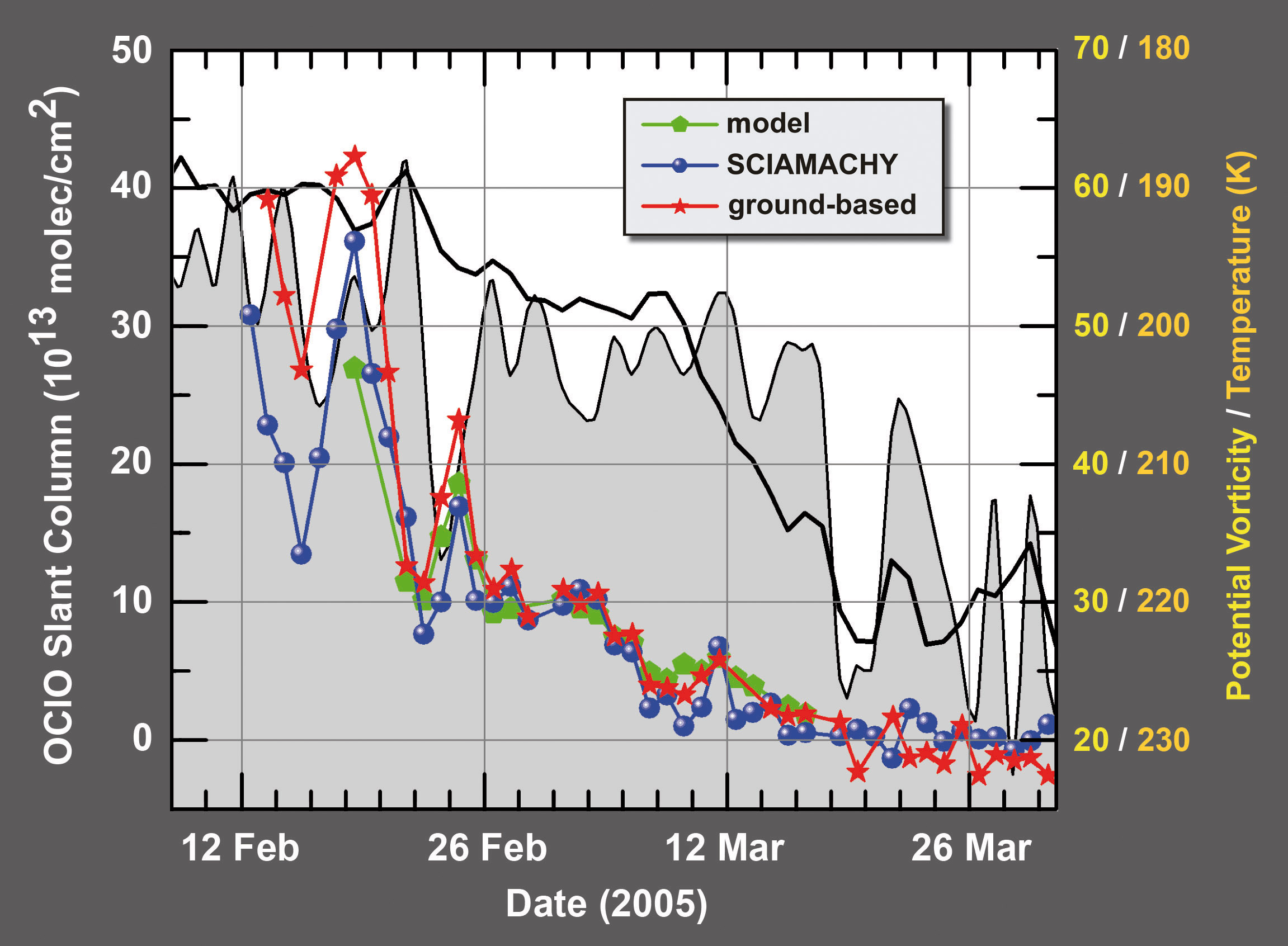
| Fig. 9-12 |
OClO slant columns retrieved from SCIAMACHY data (blue) compared with ground-based measurements (red)
sampled at the time of ENVISAT overpass over Ny-Ålesund (79°N, 12°E) in spring 2005, and model data (green).
Also shown are potential vorticity (shaded area) and temperature (black solid line) at the 475 K isentropic surface.
Courtesy: adapted from Oetjen et al. 2009) |
|
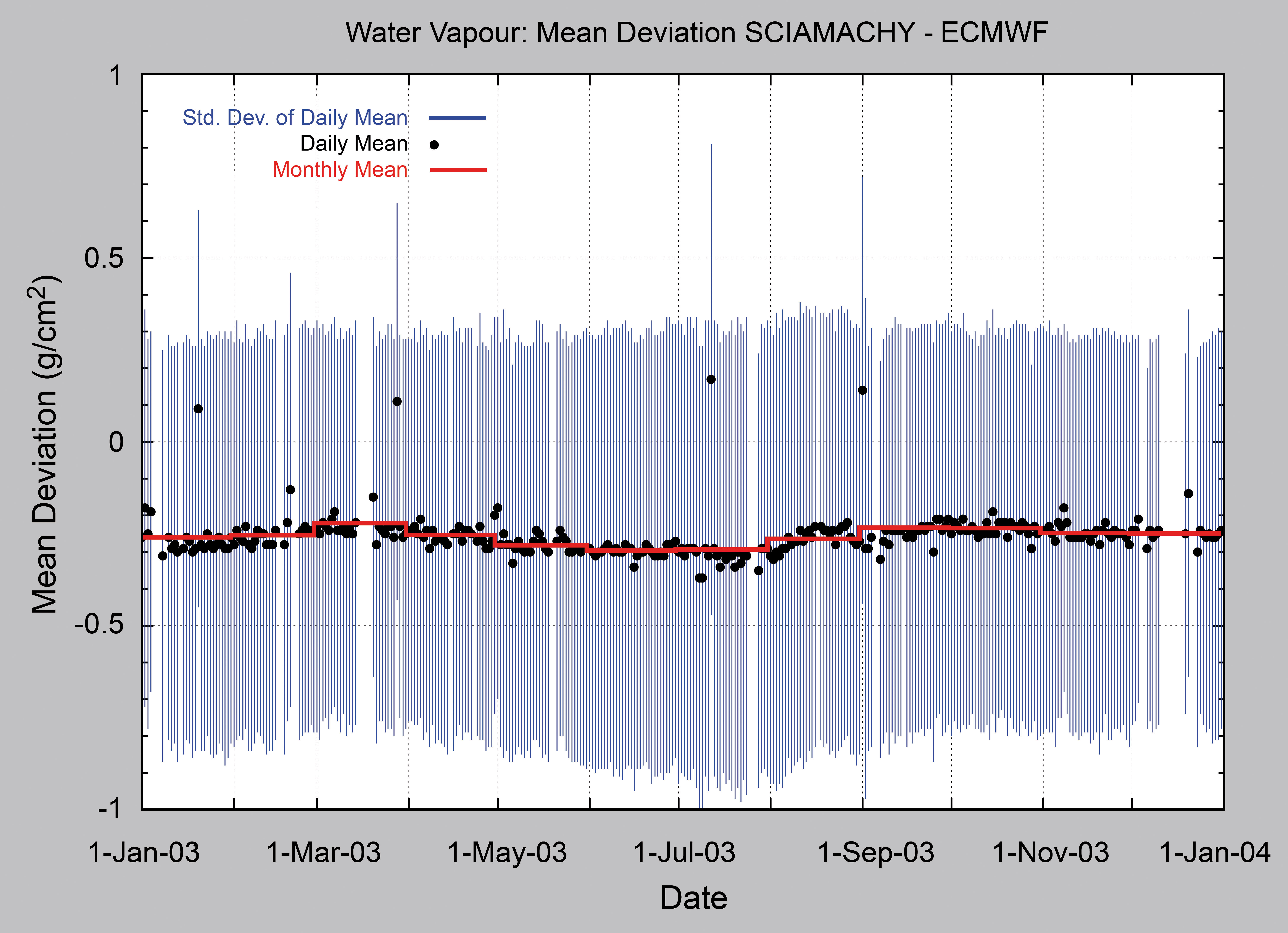
| Fig. 9-13 |
AMC-DOAS V1.0 total column water vapour compared with model data provided by the European Centre for Medium-Range
Weather Forecasts (ECMWF) over land and ocean for 2003. The comparison has been performed with co-located daily global
averages on a 0.5° × 0.5° grid (Courtesy: S. Noël, IUP-IFE, University of Bremen) |
|
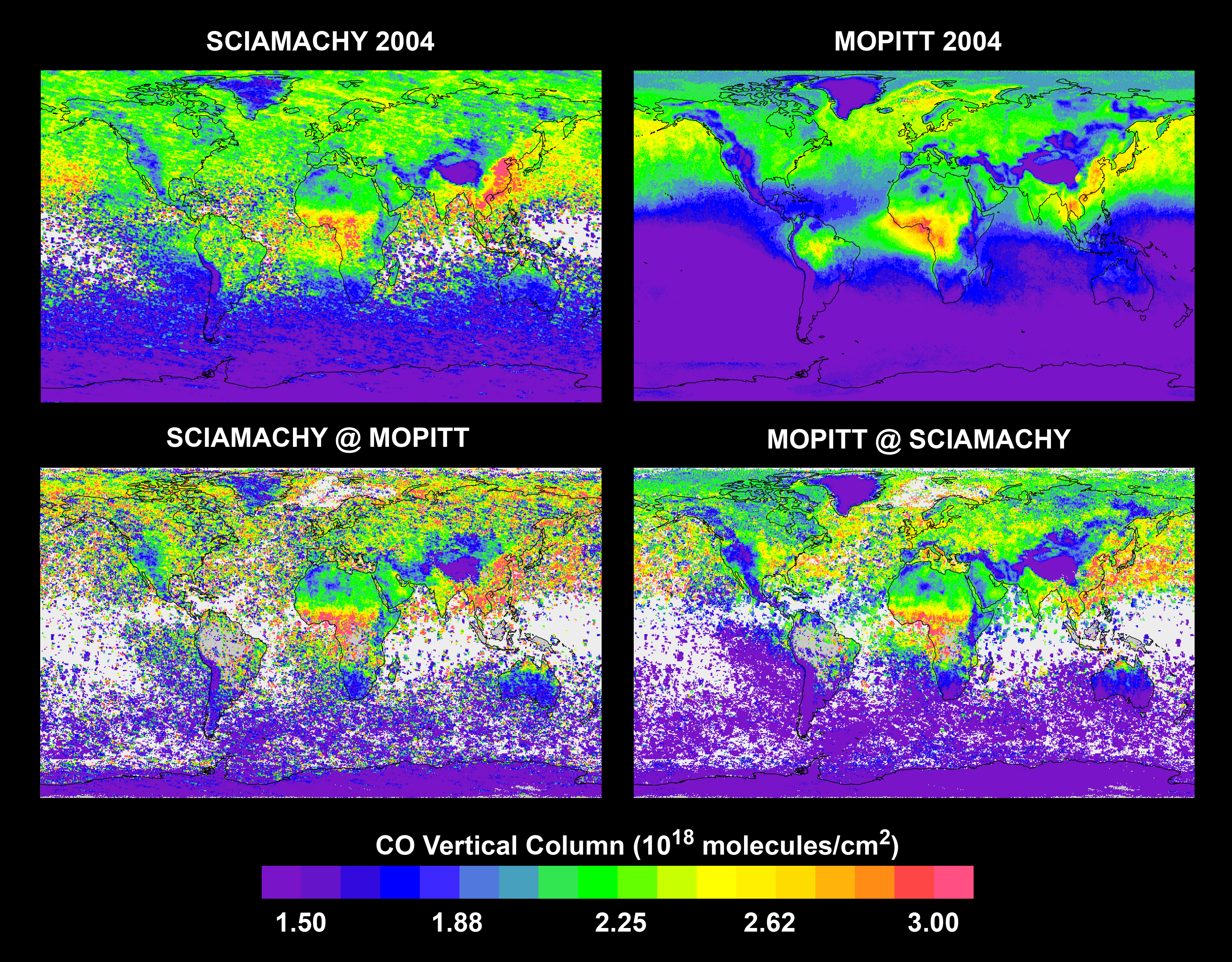
| Fig. 9-14 |
Comparison of CO vertical columns for the year 2004 derived with SCIAMACHY (top left) and MOPITT (top right).
The bottom row shows spatial coincidences between both sensors. (Courtesy: Buchwitz et al. 2007) |
 |
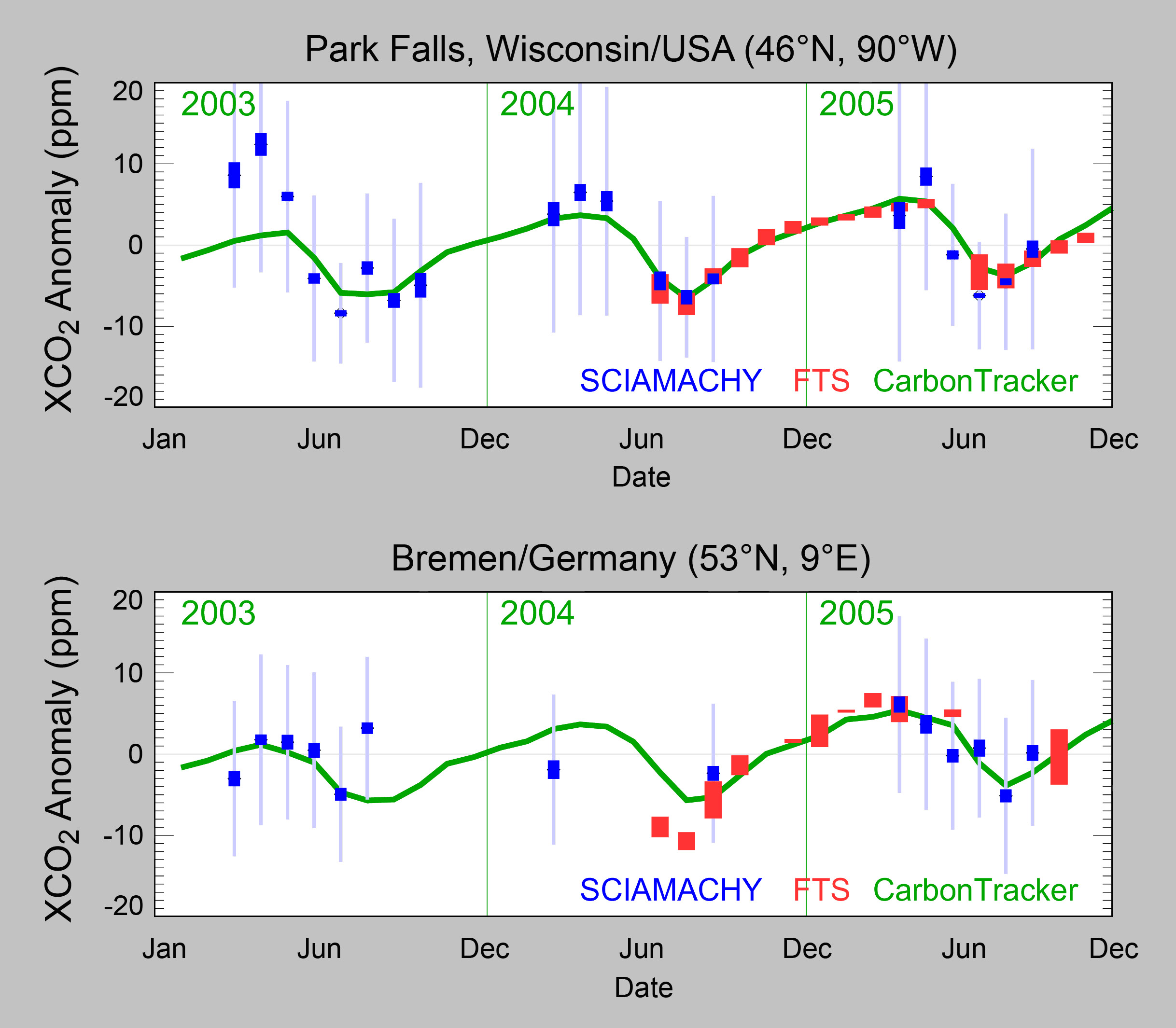
| Fig. 9-15 |
Comparison of SCIAMACHY XCO2 (blue) with ground based Fourier Transform Spectroscopy (FTS) measurements (red)
for Park Falls (top) and Bremen (bottom). Also included are corresponding CarbonTracker results (green).
Shown are comparisons of XCO2 anomalies, i.e. the corresponding mean values have been subtracted. All quality
filtered SCIAMACHY measurements within a radius of 350 km around the ground station are considered for the comparison.
(Courtesy: Schneising et al. 2008) |
 |
| Fig. 9-16 |
Zonal mean O3 from SCIAMACHY vertical profiles averaged from 2005 to 2008. Only co-located daily
measurements with MLS have been used, where the criteria for co-locations are 100 km spatial and 10
hours temporal difference. Co-locations with MLS measurements during night with solar zenith angles > 90°
have been excluded. (Courtesy: S. Mieruch, IUP-IFE, University of Bremen) |

|
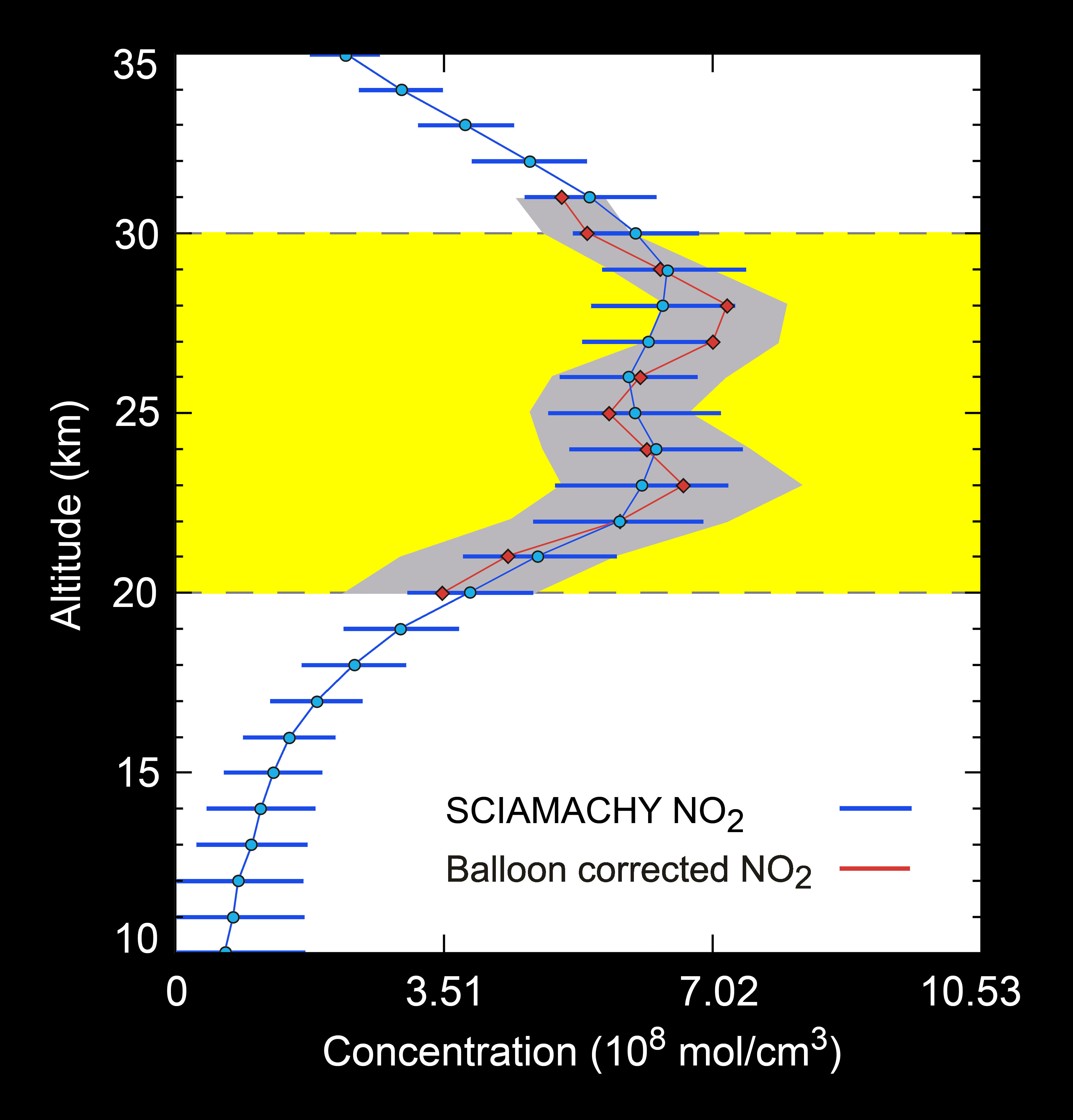
| Fig. 9-17 |
Comparison between a SCIAMACHY NO2 profile (blue) retrieved with the SCIATRAN V3.1 algorithm and
co-located balloon NO2 measurements at Kiruna (red). The grey shaded area shows the uncertainty of
the balloon measurements, whereas the yellow region indicates the altitude range where both instruments
are considered to probe similar air masses. (Courtesy: R. Bauer IUP-IFE, University of Bremen) |
|
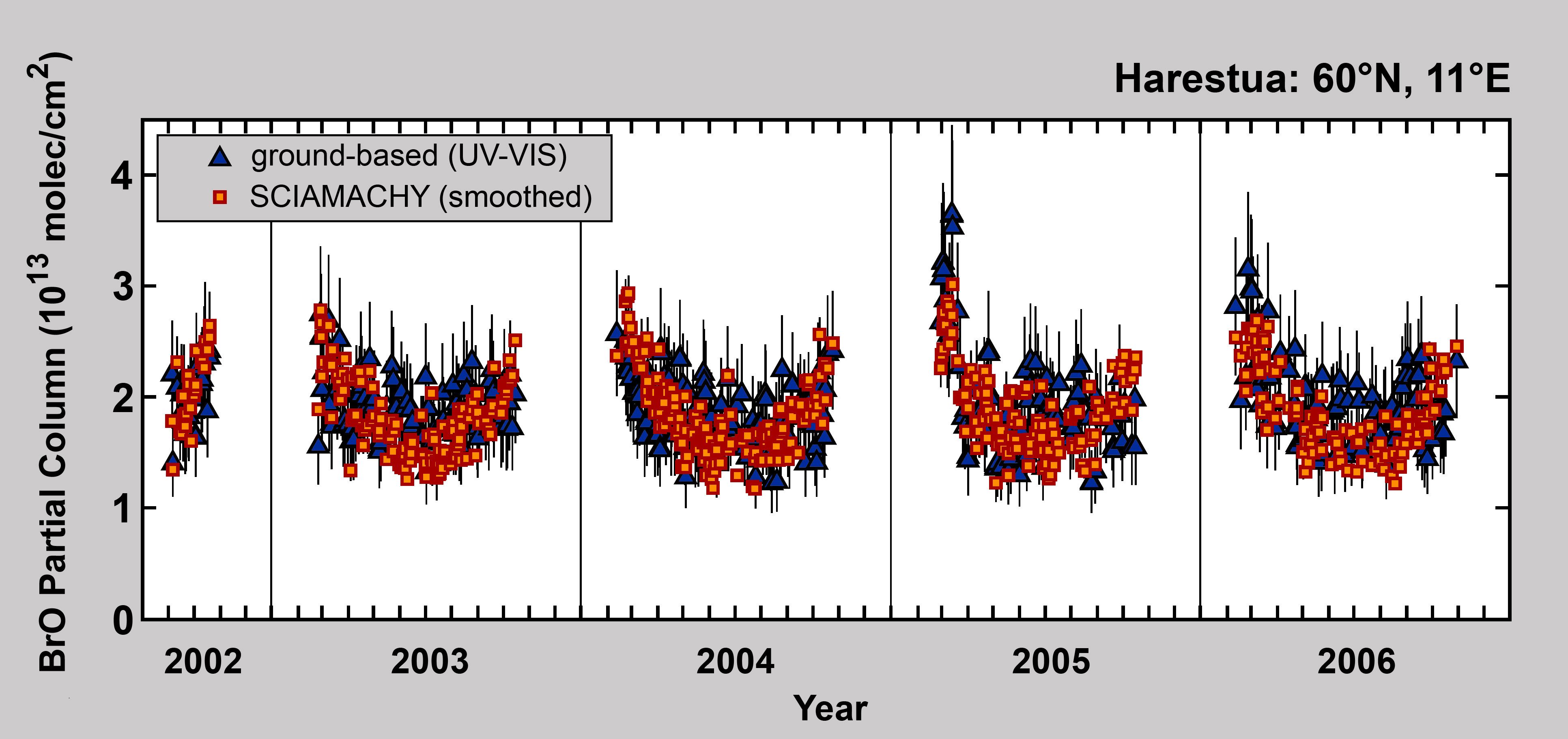
| Fig. 9-18 |
Intercomparison of the 15-27 km BrO partial columns calculated from SCIAMACHY limb and ground-based UV-VIS
profiles at Harestua/Norway for 2002-2006 (morning coincidences). To reduce comparison errors due to differences
in vertical smoothing of the vertical profile, SCIAMACHY profiles were smoothed using coincident ground-based UV-VIS
averaging kernels. (Courtesy: adapted from Hendrick et al. 2009) |
|
Page generated 31 August 2011