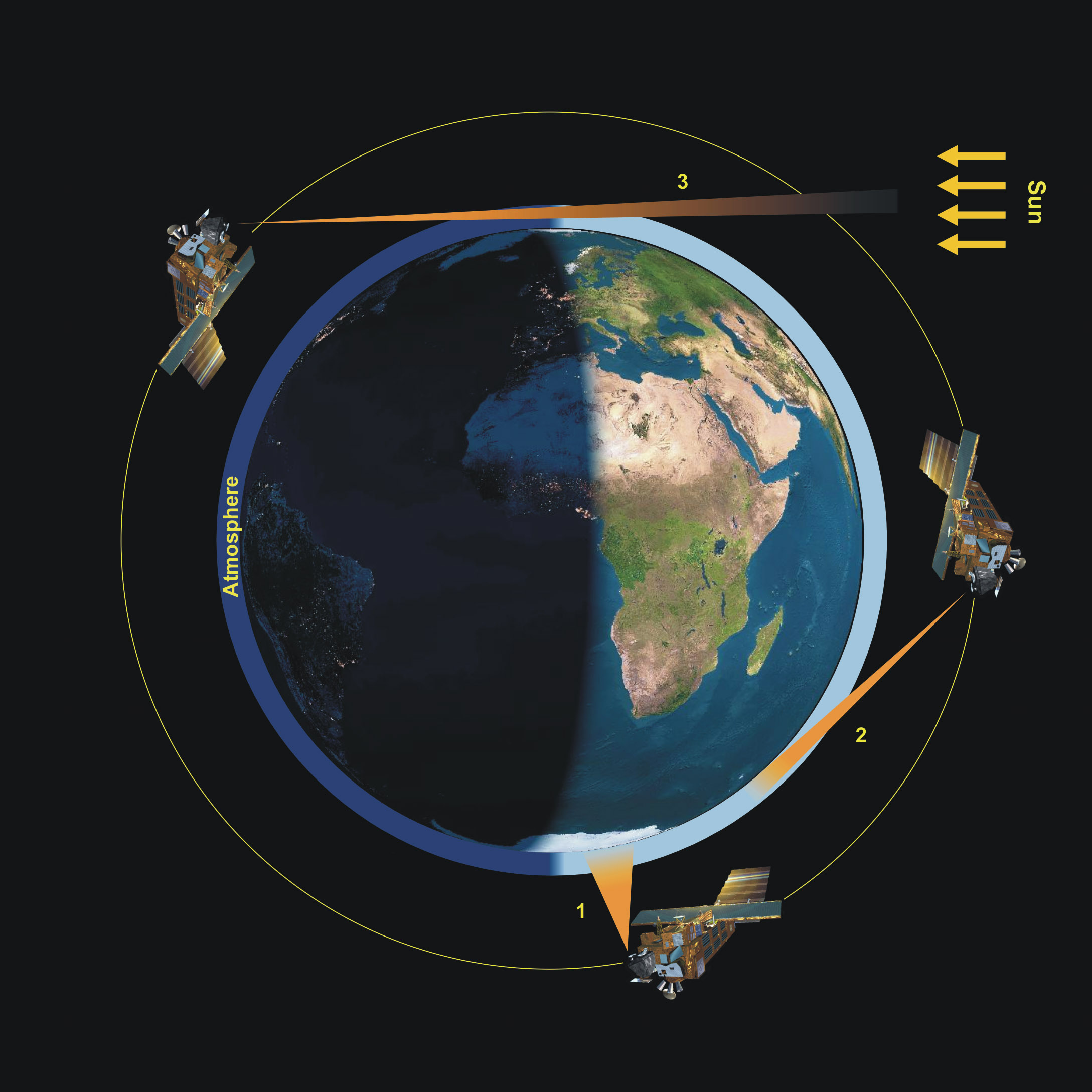
| Fig. 4-1 |
SCIAMACHY's scientific observation modes: 1 = nadir, 2 = limb, 3 = occultation. (Courtesy: DLR-IMF) |
|
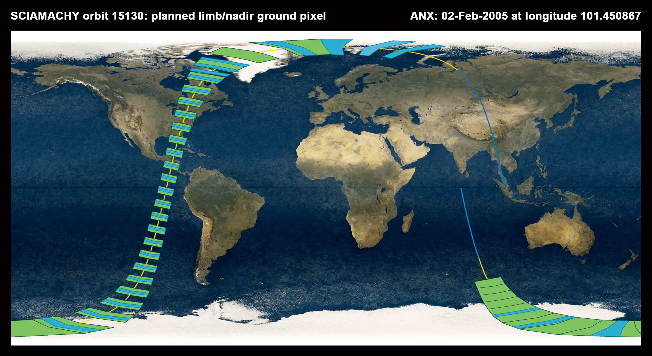
| Fig. 4-2 |
An orbit with planned limb/nadir matching on the dayside of the orbit.
The sequence of nadir and limb states in a timeline is arranged such that limb ground pixels (blue),
defined by the line-of-sight tangent point, fall right into a nadir ground pixel (green) in the illuminated part of the orbit.
(Courtesy: DLR-IMF/SRON)
|
|
| Fig. 4-3 |
ENVISAT's yaw steering, the yaw steering correction of limb states and the resulting SCIAMACHY yaw steering.
Between ENVISAT and SCIAMACHY yaw steering, an orbital shift
of 27° exists which reflects the observation geometry in elevation when looking to the horizon in flight direction.
Courtesy: DLR-IMF) |

|
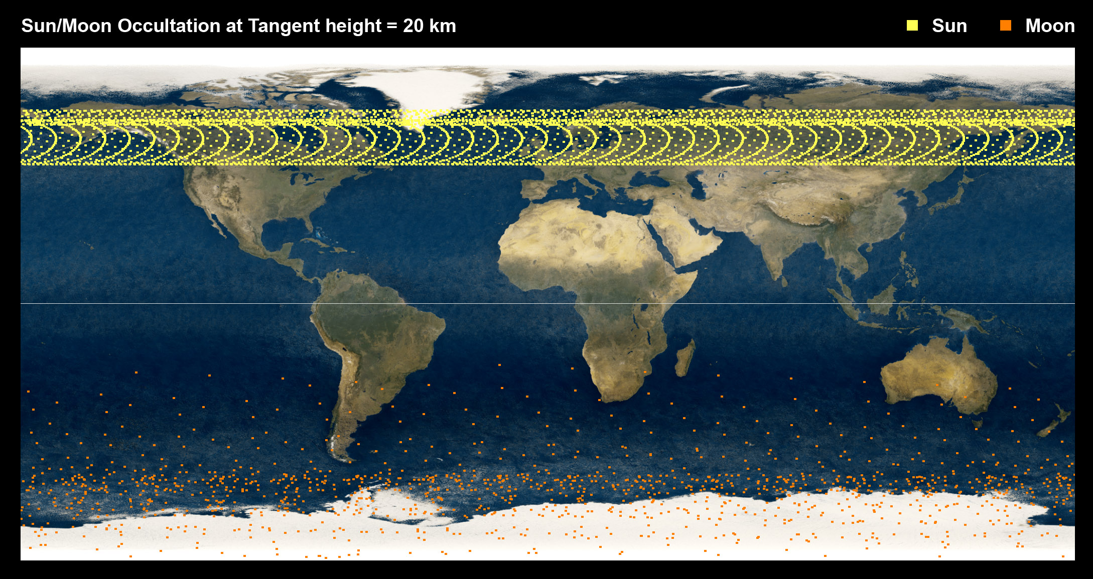
| Fig. 4-4 |
Tangent point geolocation at an altitude of 20 km for all solar and lunar occultation measurements in the year 2009.
(Courtesy: DLR-IMF/SRON) |
|
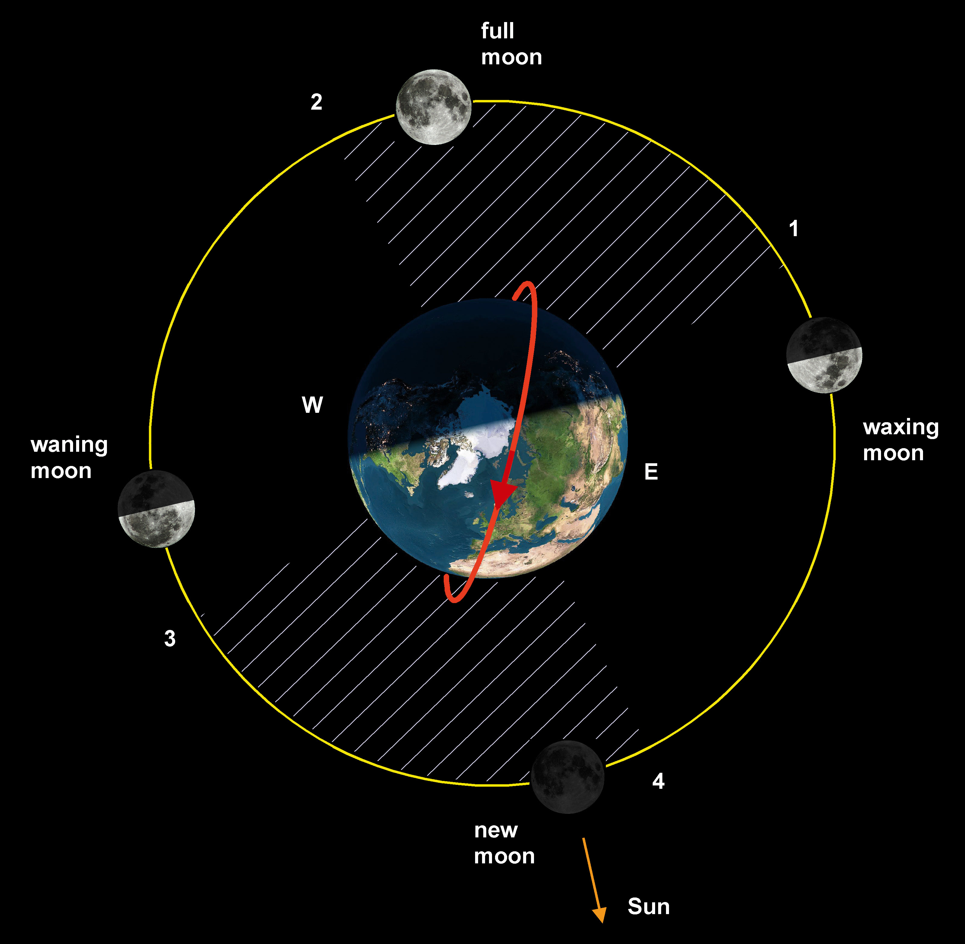
| Fig. 4-5 |
SCIAMACHY's monthly lunar visibility occurs between 1 and 2 over the southern hemisphere (lunar phase > 0.5).
The hatched area illustrates the limb TCFoV of 88°. Visibility at smaller lunar phases over the northern
hemisphere between 3 and 4 is not used because it coincides with solar occultations. (Courtesy: DLR-IMF) |
|
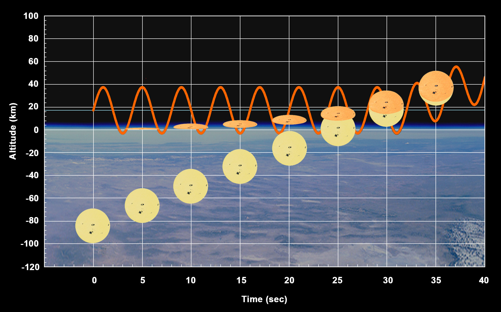
| Fig. 4-6 |
The effect of refraction during sunrise. The position of the Sun is indicated by the yellow disk while the distorted refracted
image appears above the horizon. About 30 sec after begin of sunrise the position of the true and refracted disk overlap
and refraction becomes negligible. The sinusoidal curve illustrates the elevation scan of the ESM at the start of the Sun
occultation states. (Courtesy: DLR-IMF; background photo: NASA Johnson Space Center and Image Science & Analysis Laboratory) |
|
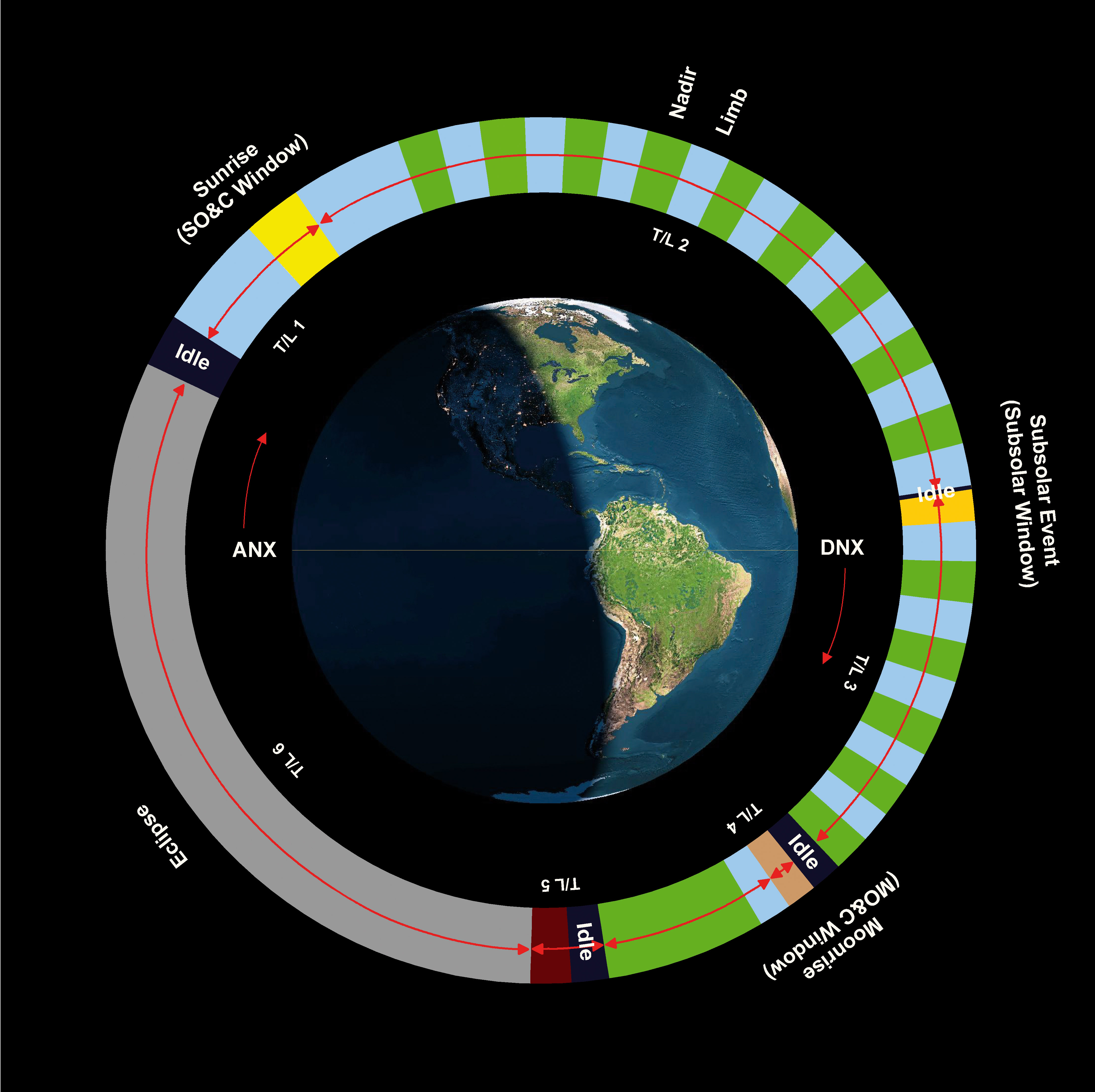
| Fig. 4-7 |
SCIAMACHY reference orbit with Sun/Moon fixed events along the orbit. The events define orbital segments which are filled with timelines.
State duration is not to scale. (Courtesy: DLR-IMF) |
|
| Fig. 4-8 |
Nadir coverage after 1 day of routine measurements. At the equator consecutive nadir ground pixels are separated by about 1600 km.
This gap is filled within 3 days in case of nadir only state sequences. With successive limb/nadir states, full nadir coverage
at the equator requires 6 days. (Courtesy: DLR-IMF/ SRON) |

|
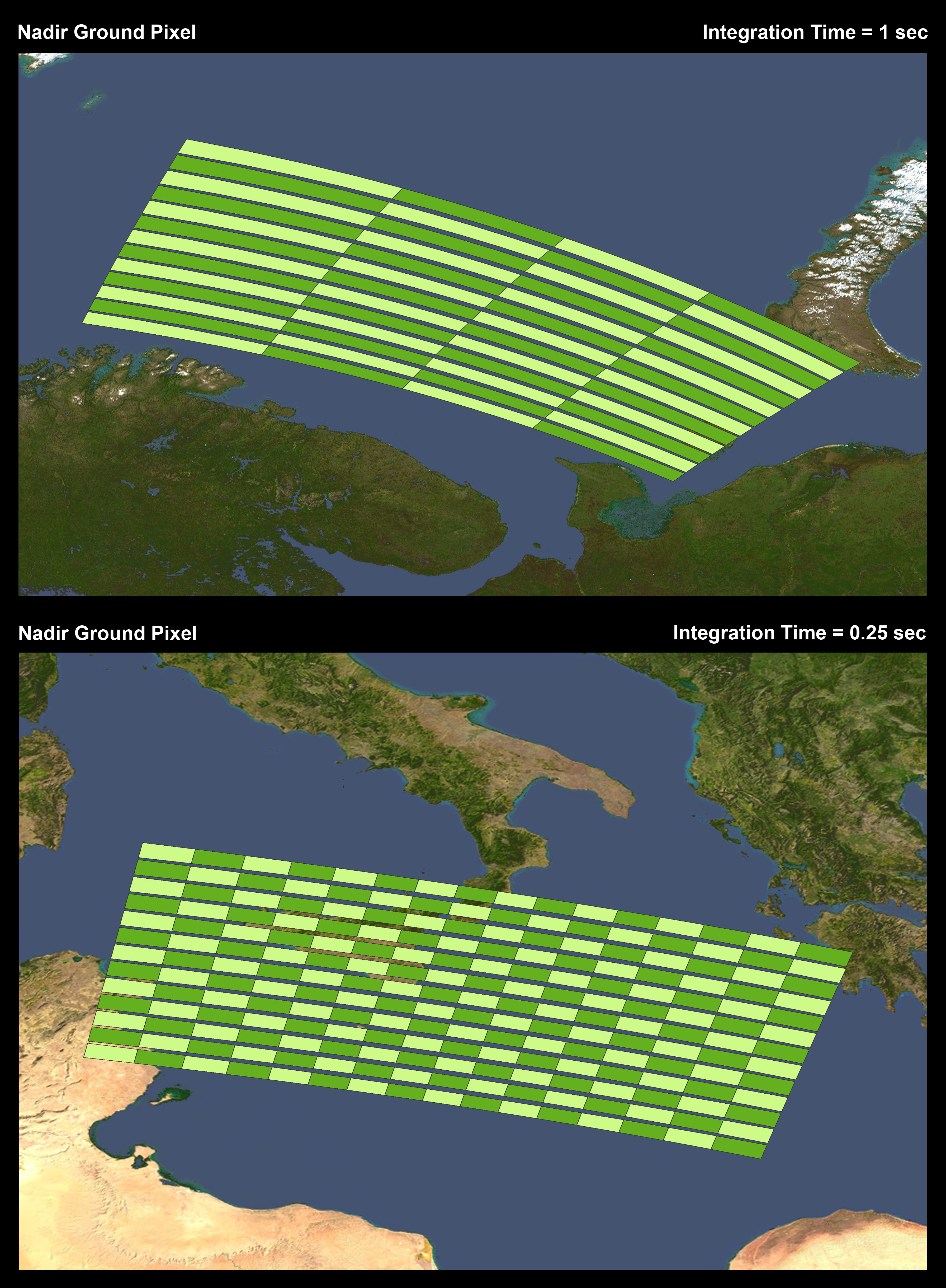
| Fig. 4-9 |
The pattern of ground pixels in a nadir measurement for an integration time of 1 sec (top) and 250 msec (bottom). Only the forward scans are shown.
This causes the along-track gaps between consecutive scans which vary in width due to a projection effect.
Across-track extent is defined by the integration time while along-track the size reflects the dimension of the
IFoV with only a small contribution of the integration time. (Courtesy: DLR-IMF; background maps: NASA) |
|
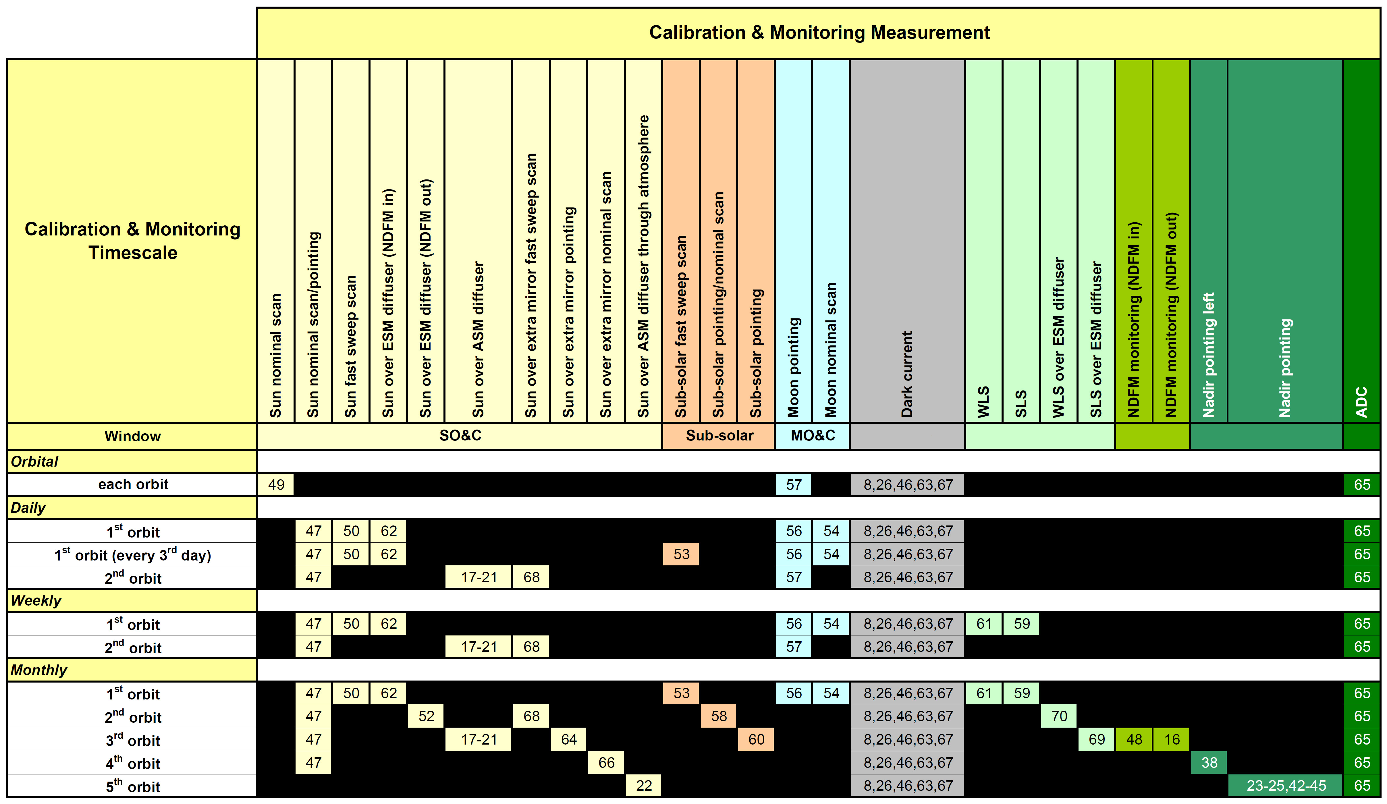
| Fig. 4-10 |
Calibration and monitoring scenarios from orbital to monthly timescales. In the top row the
individual measurements and their targets, e.g. Sun, Moon, lamps, are listed. The states used
in each calibration orbit refer to the definitions in Table 4-2. All states unrelated to the Sun or the Moon
can be executed several times at any position along the orbit. (Courtesy: DLR-IMF) |
|
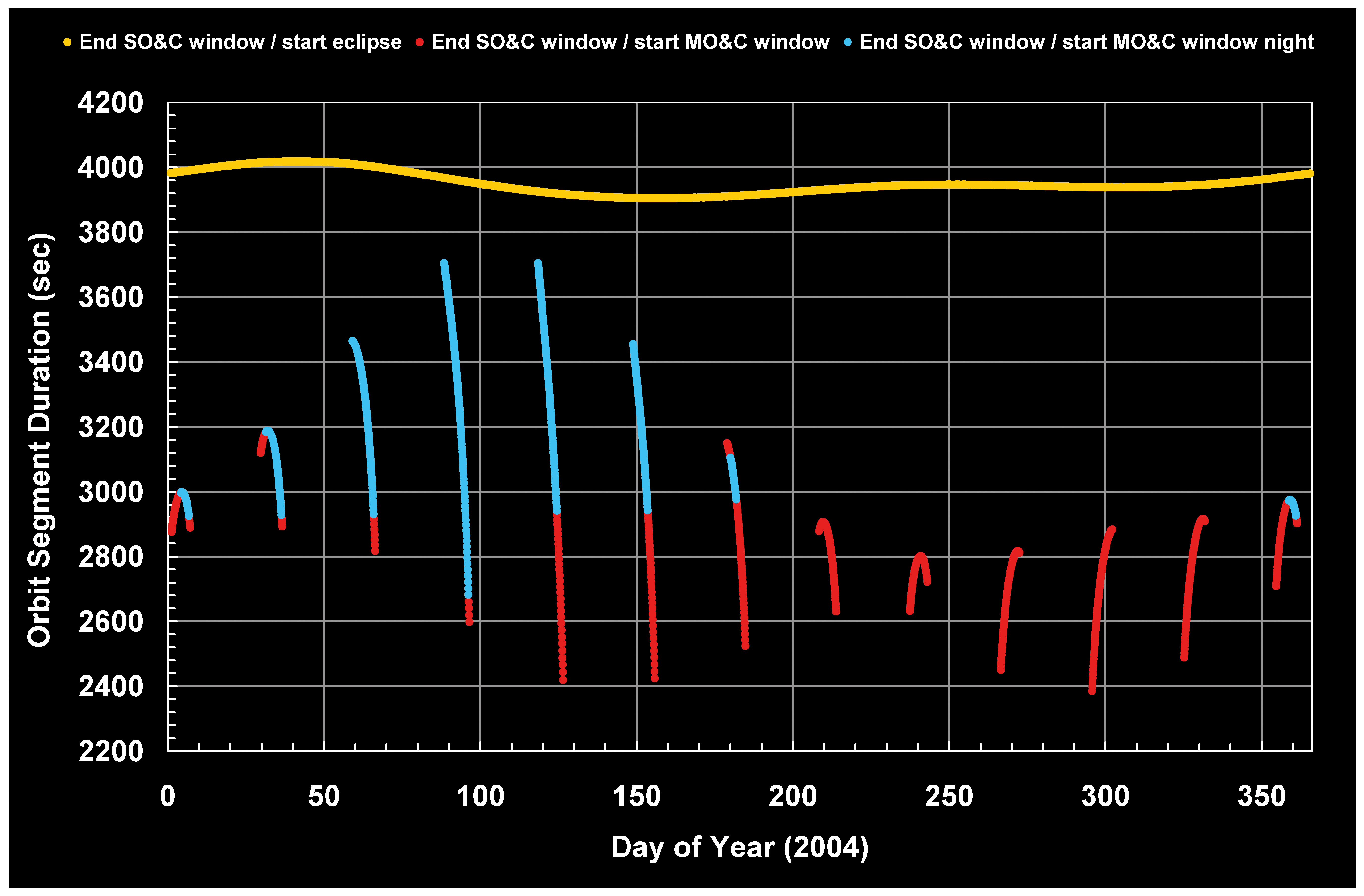
| Fig. 4-11 |
Example of the seasonal temporal variability of orbital segments for the year 2004.
The time interval between end of SO&C window and start of eclipse varies only slightly over a year (yellow).
In the monthly lunar visibility periods, the time between end of MO&C window and start of eclipse shows a much higher
variation (red curves). The blue segments indicate lunar visibility phases where moonrise occurs on the nightside,
i.e. those which can be used for occultations. (Courtesy: DLR-IMF) |
|
Page generated 31 August 2007