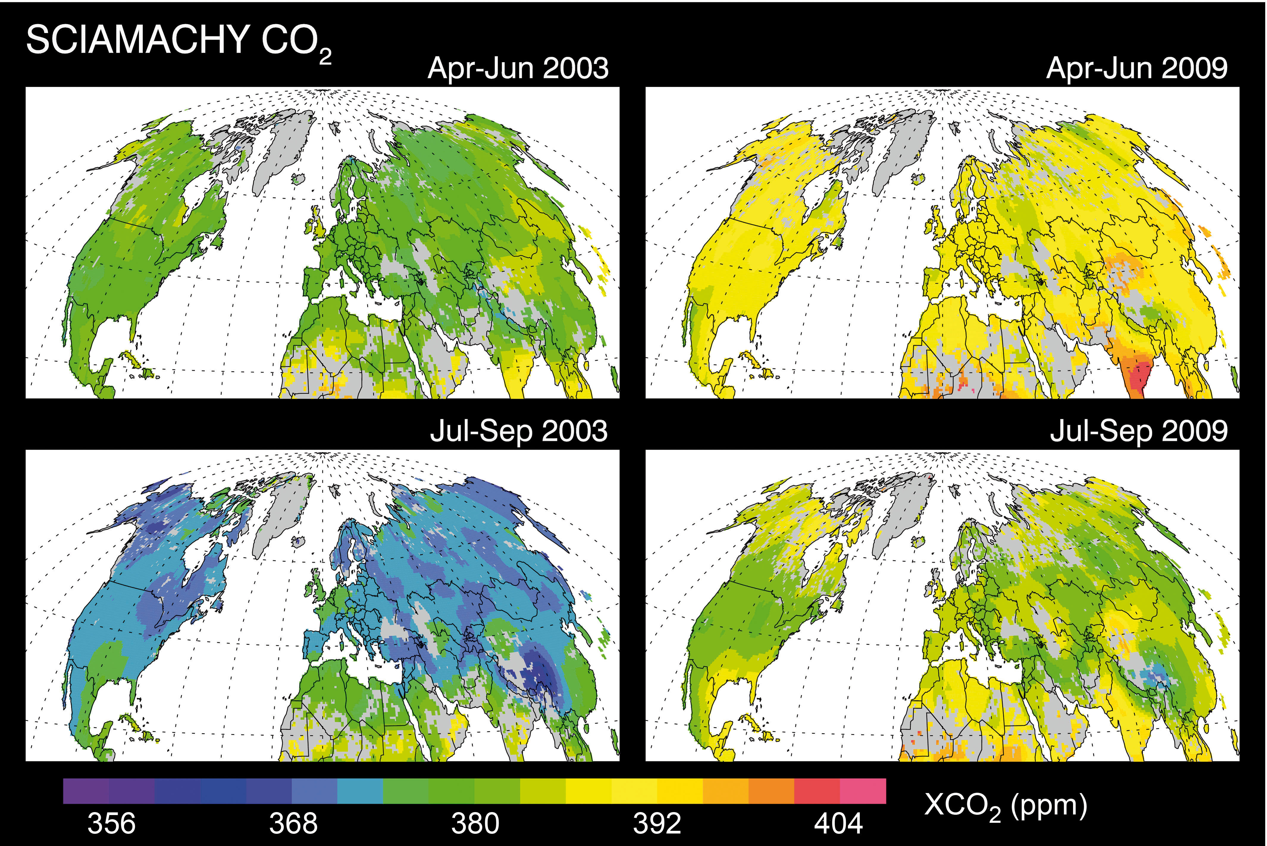
| Fig. 10-1 |
Northern hemispheric CO2 distribution as observed by SCIAMACHY. The differences between spring and summer
are due to the CO2 'breathing' of the vegetation. (Courtesy: M. Buchwitz, IUP-IFE, University of Bremen) |
|
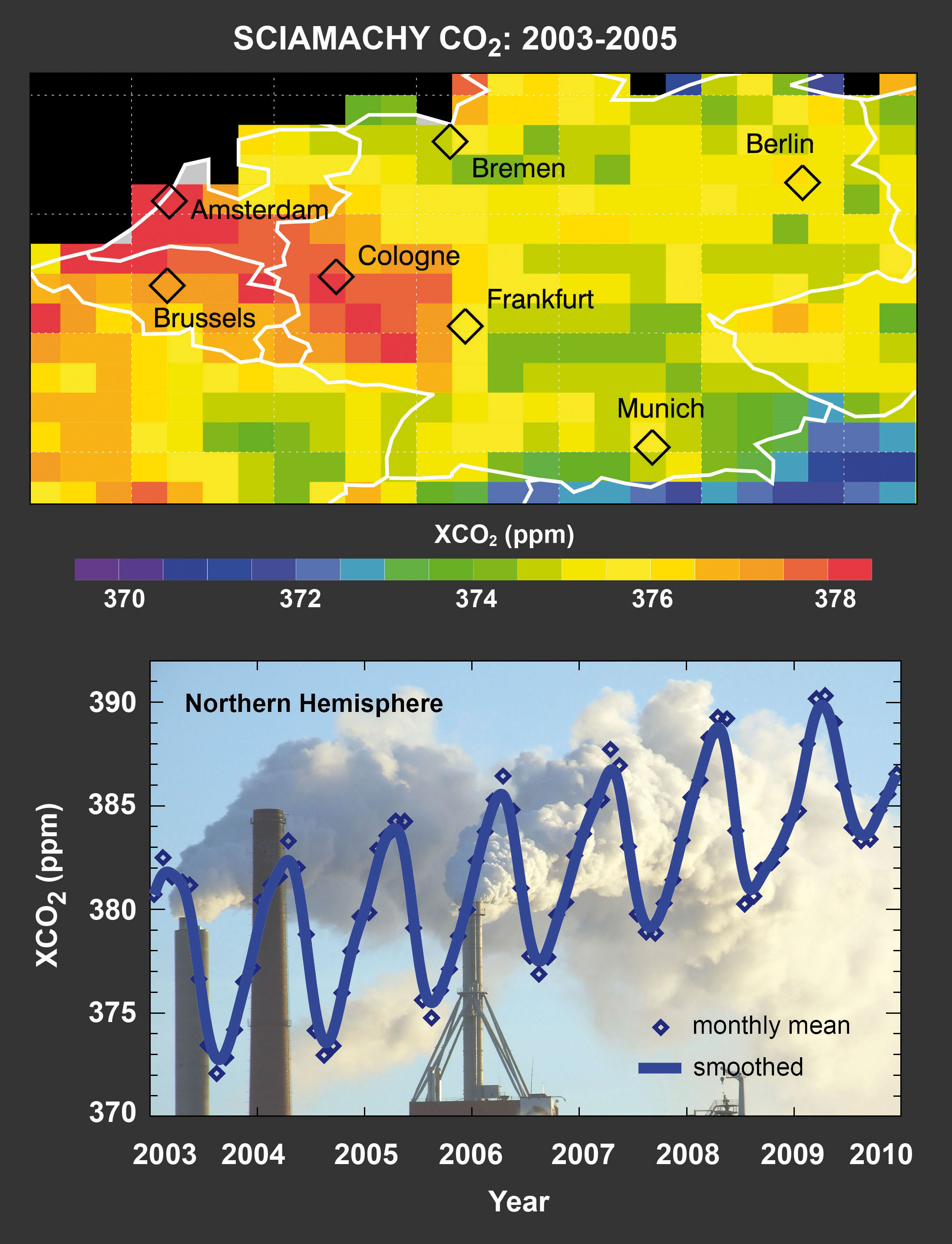
| Fig. 10-2 |
Top: Elevated CO2 (shown in red) as observed by SCIAMACHY over Central Europe's most populated Rhine-Main area.
Bottom: Increase of Northern hemispheric CO2 derived from SCIAMACHY measurements. (Courtesy: M. Buchwitz, IUP-IFE, University of Bremen) |
|
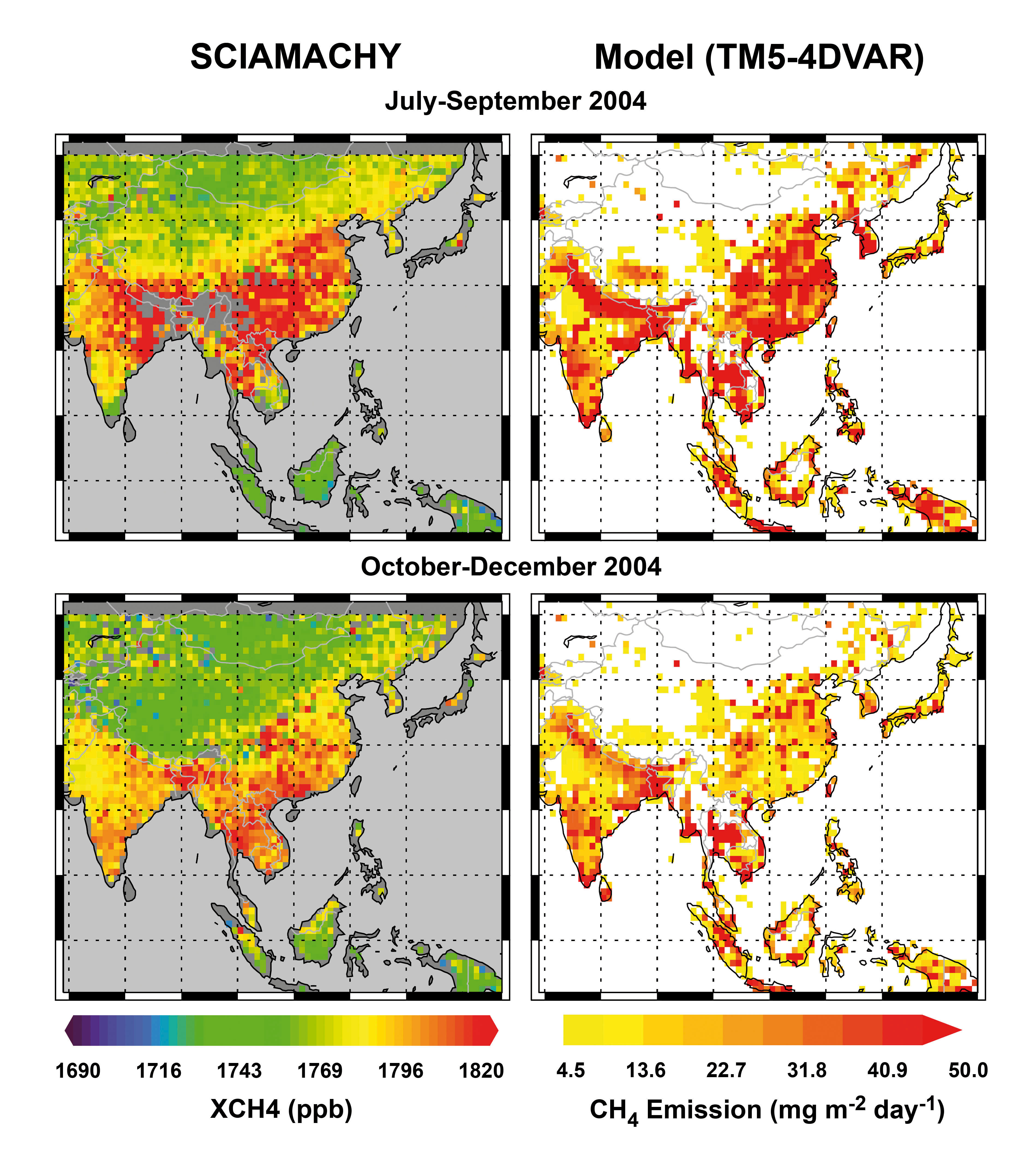
| Fig. 10-3 |
Methane emission derived from SCIAMACHY data. Left column: Column-averaged CH4 mixing ratios (XCH4)
over South-East Asia from SCIAMACHY for summer and autumn 2004. Right column: Modelled emissions per
1° × 1° grid cell. (Courtesy: adapted from Bergamaschi et al. 2009, reproduced by permission of American
Geophysical Union) |
|
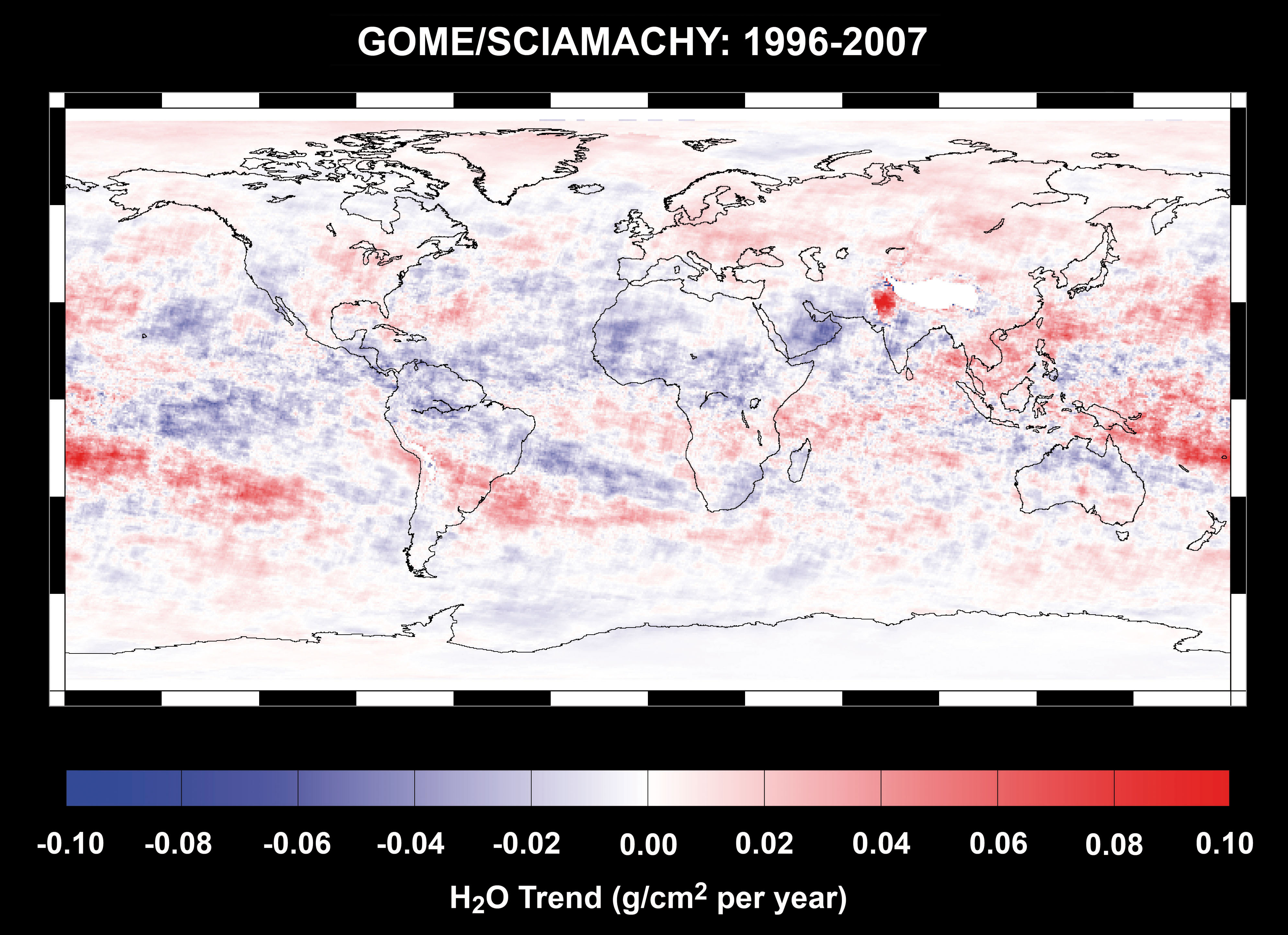
| Fig. 10-4 |
Water vapour trends for 1996 to 2007 as derived from GOME and SCIAMACHY. (Courtesy: S. Mieruch, IUP-IFE,
University of Bremen) |
|
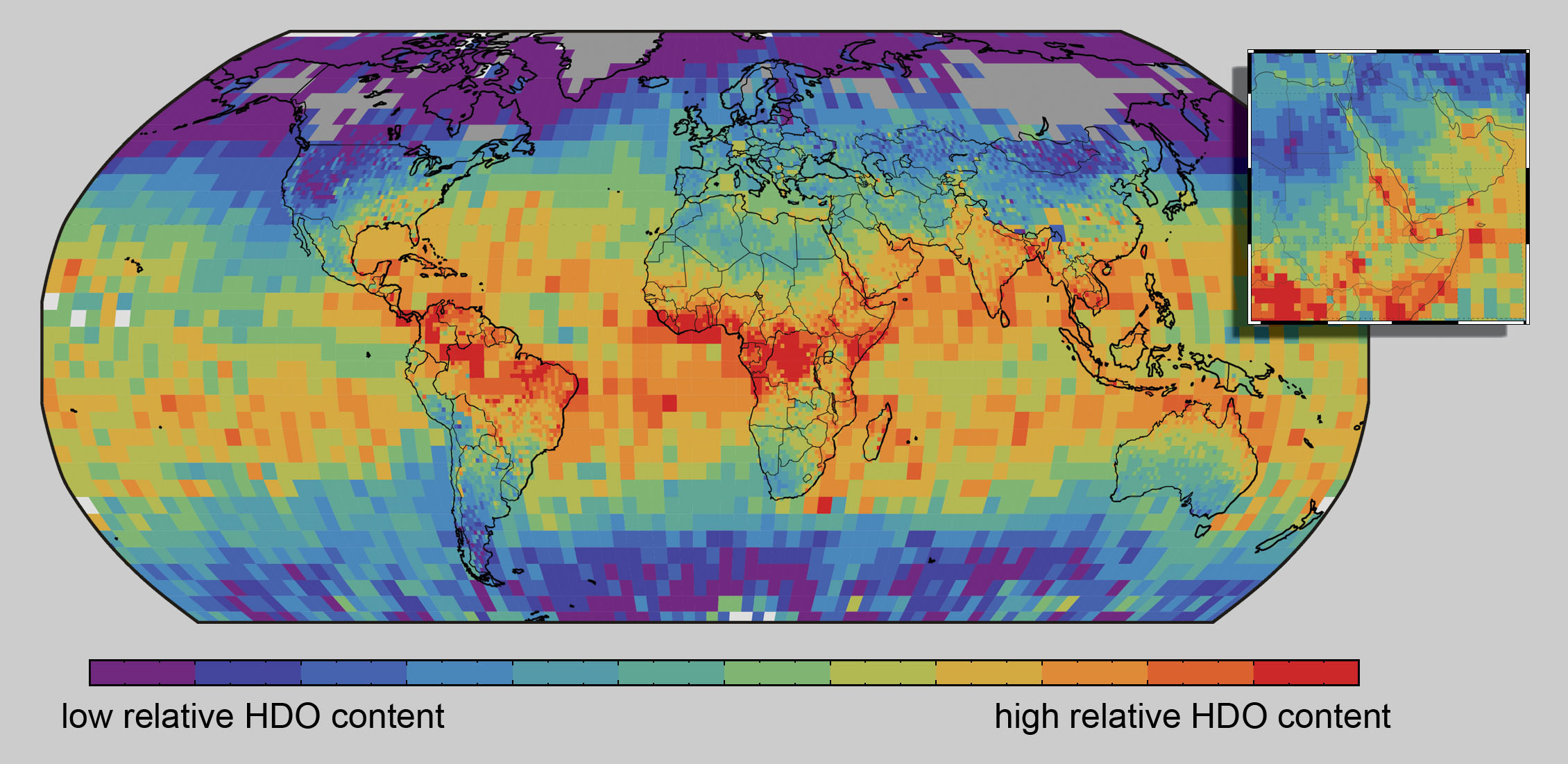
| Fig. 10-5 |
Global distribution of the water isotope HDO shown as relative abundance of water vapour averaged between 2003 and 2005.
The inset displays enhanced HDO fractions due to strong evaporation over the Red Sea (Courtesy: C. Frankenberg, SRON - now JPL) |
|
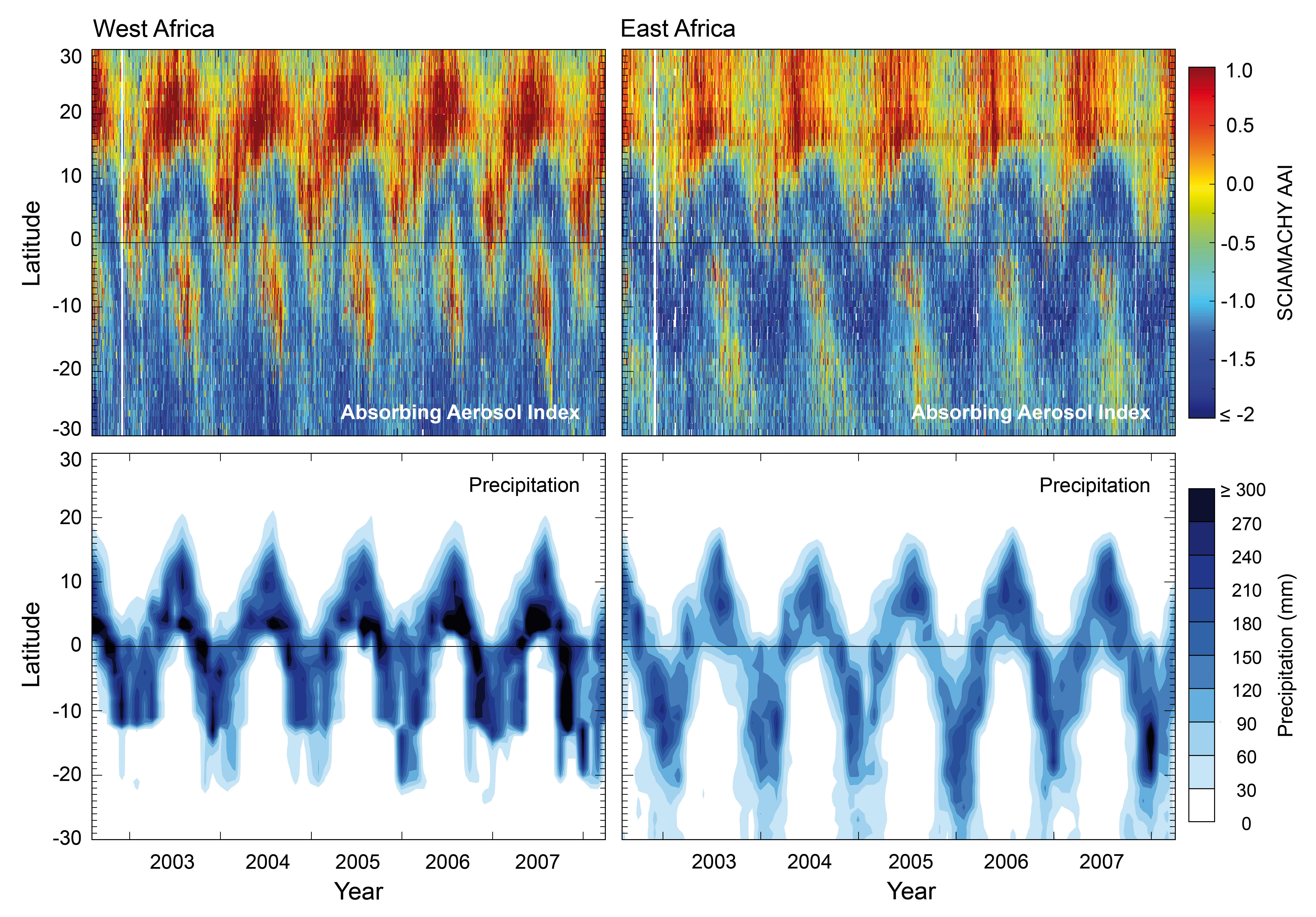
| Fig. 10-6 |
Zonally averaged AAI from SCIAMACHY for each day between August 2002 and April 2008 as a function of
latitude in Western and Eastern Africa (upper panels). The bottom panels display the monthly and zonally
averaged precipitation for the same areas and the same period. (Courtesy: M. de Graaf, KNMI) |
|
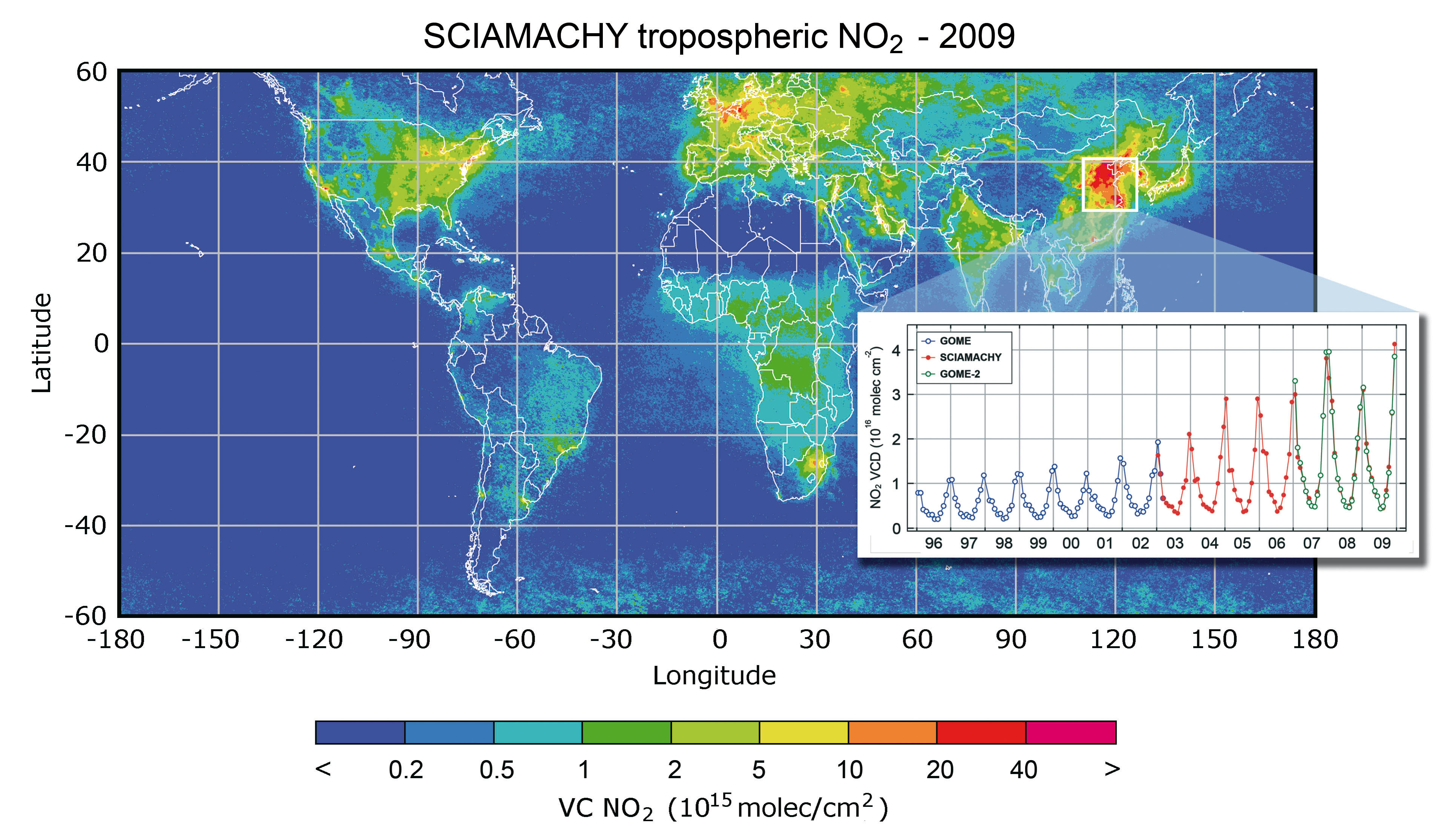
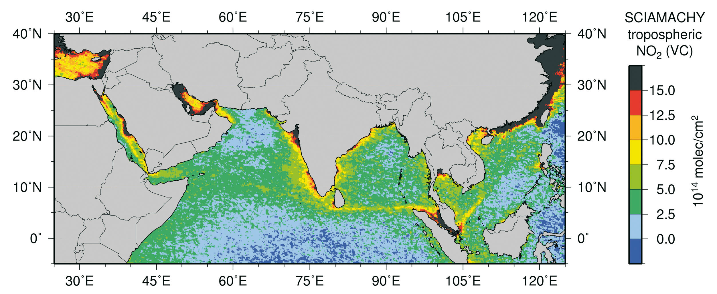
| Fig. 10-7 |
Global survey of tropospheric vertical column (VC) NO2 for 2009. Clearly visible are the industrialised regions
in the northern hemisphere and the regions of biomass burning in the southern hemisphere. The inset illustrates how
NO2 concentrations have risen in China from 1996-2009. The trend analysis uses data from GOME (1996-2002) and
SCIAMACHY (2003-2009). While 'old' industrialised countries were able to stop the increase of NO2 emissions,
the economical growth in China turns out to be a strong motor for pollution.
(Courtesy: A. Richter, IUP-IFE, University of Bremen) |
|
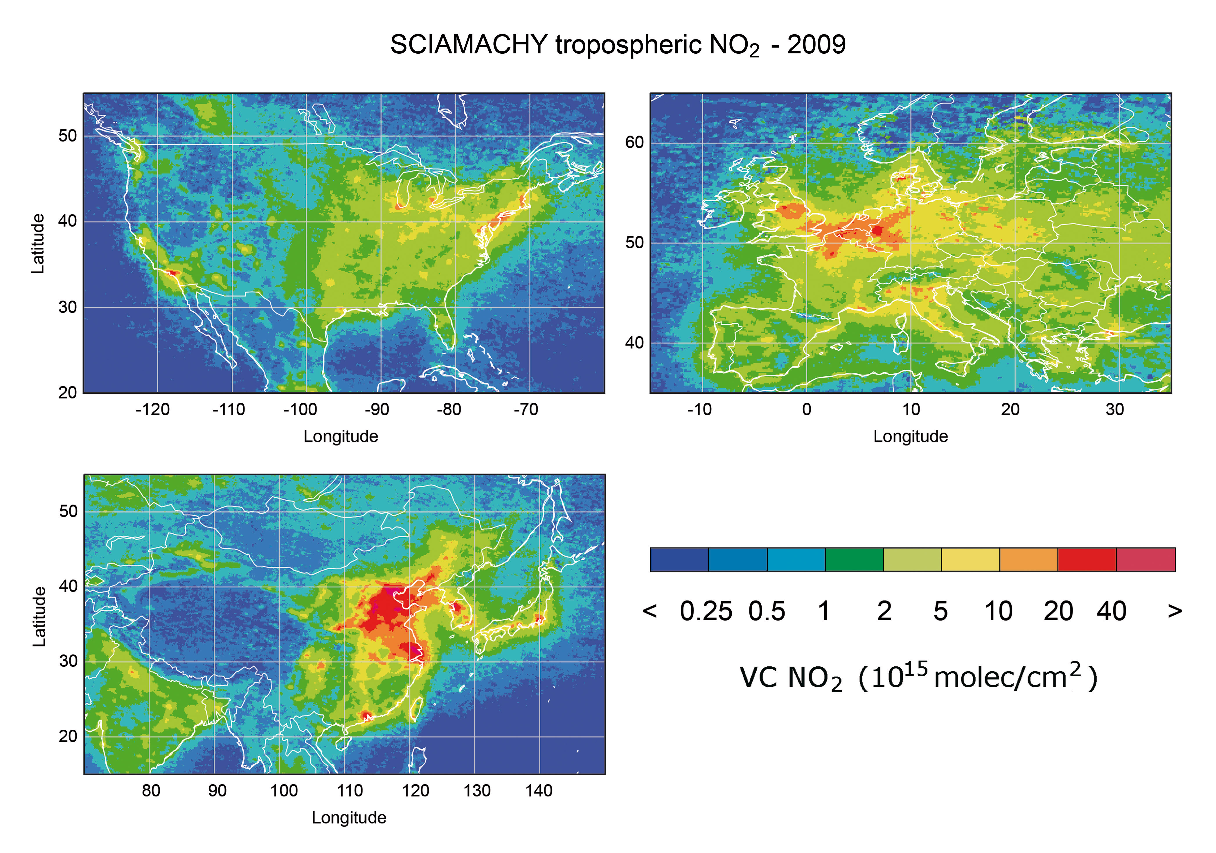
| Fig. 10-8 |
Mean tropospheric vertical column (VC) NO2 densities over Europe, the United States and China in 2009.
(Courtesy: A. Richter, IUP-IFE, University of Bremen) |
|
| Fig. 10-9 |
NO2 densities over the Indian Ocean and the Red Sea as derived from measurements between August 2002 and April 2004.
Ship routes from Eastern Asia to the Suez Canal can be clearly seen. Along the industrialised coast lines,
strong NO2 concentrations are related to urban areas. (Courtesy: A. Richter, IUP-IFE, University of Bremen) |
|
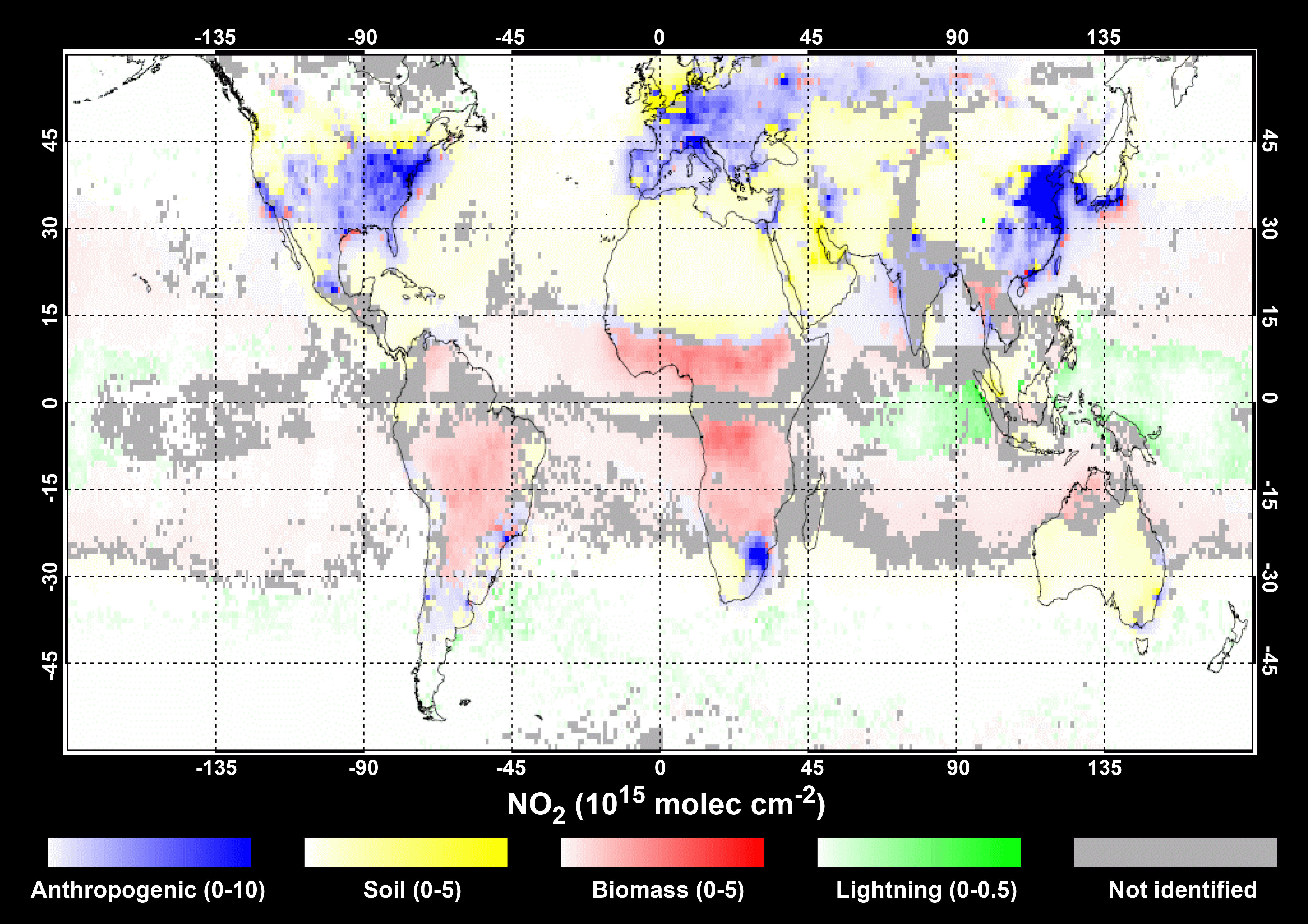
| Fig. 10-10 |
Dominant NOx source identification based on analyses of the time series of measured tropospheric NO2 from GOME and
SCIAMACHY satellite observations (1996-2006). (Courtesy: van der A et al. 2008, reproduced by permission of the
American Geophysical Union) |
|
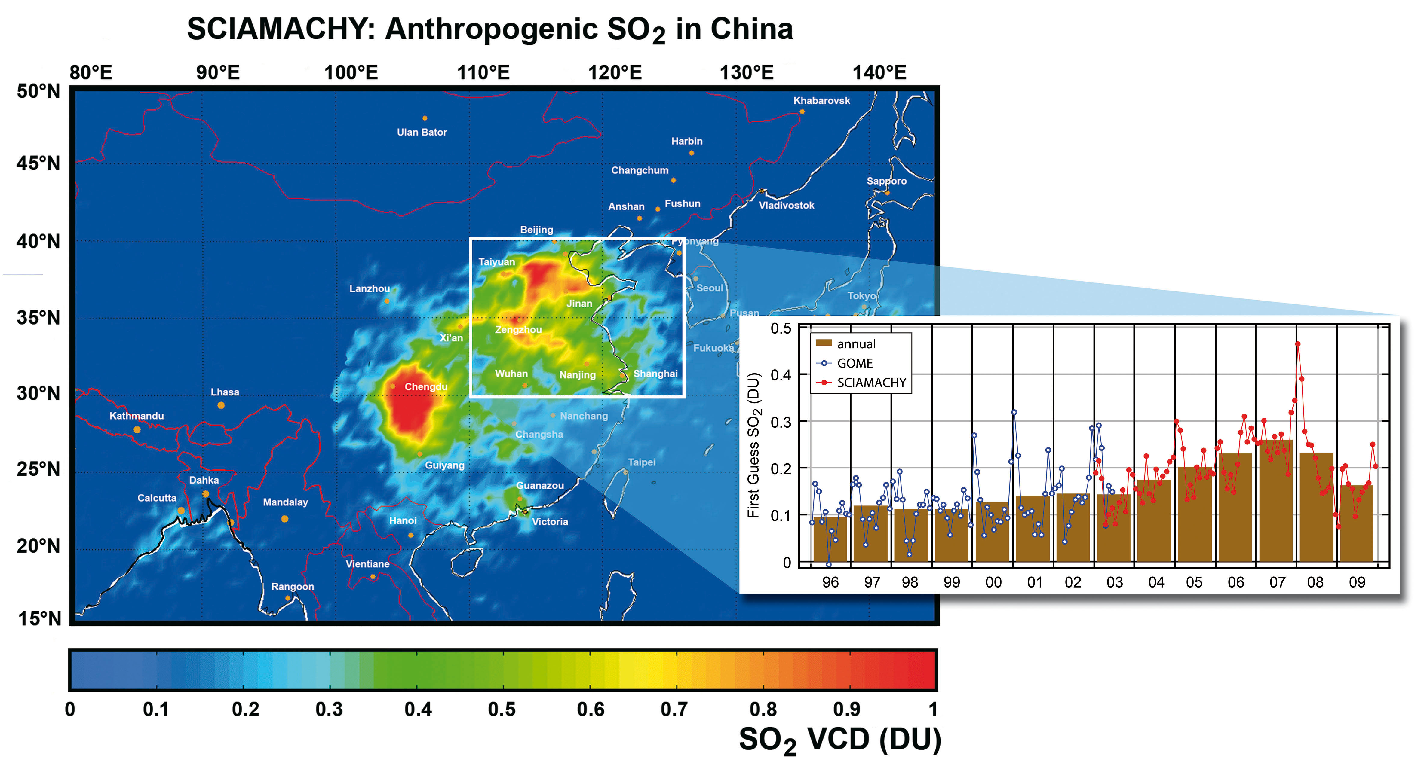
| Fig. 10-11 |
Average SO2 vertical column densities (VCD) over eastern China during the year 2003. SCIAMACHY's improved
spatial resolution permits to identify localised emissions due to anthropogenic activities. The trend analysis
uses data from GOME (1996-2002) and SCIAMACHY (2003-2009).
(Courtesy: map - M. Van Roozendael, BIRA-IASB; trend - A. Richter, IUP-IFE, University of Bremen) |
|
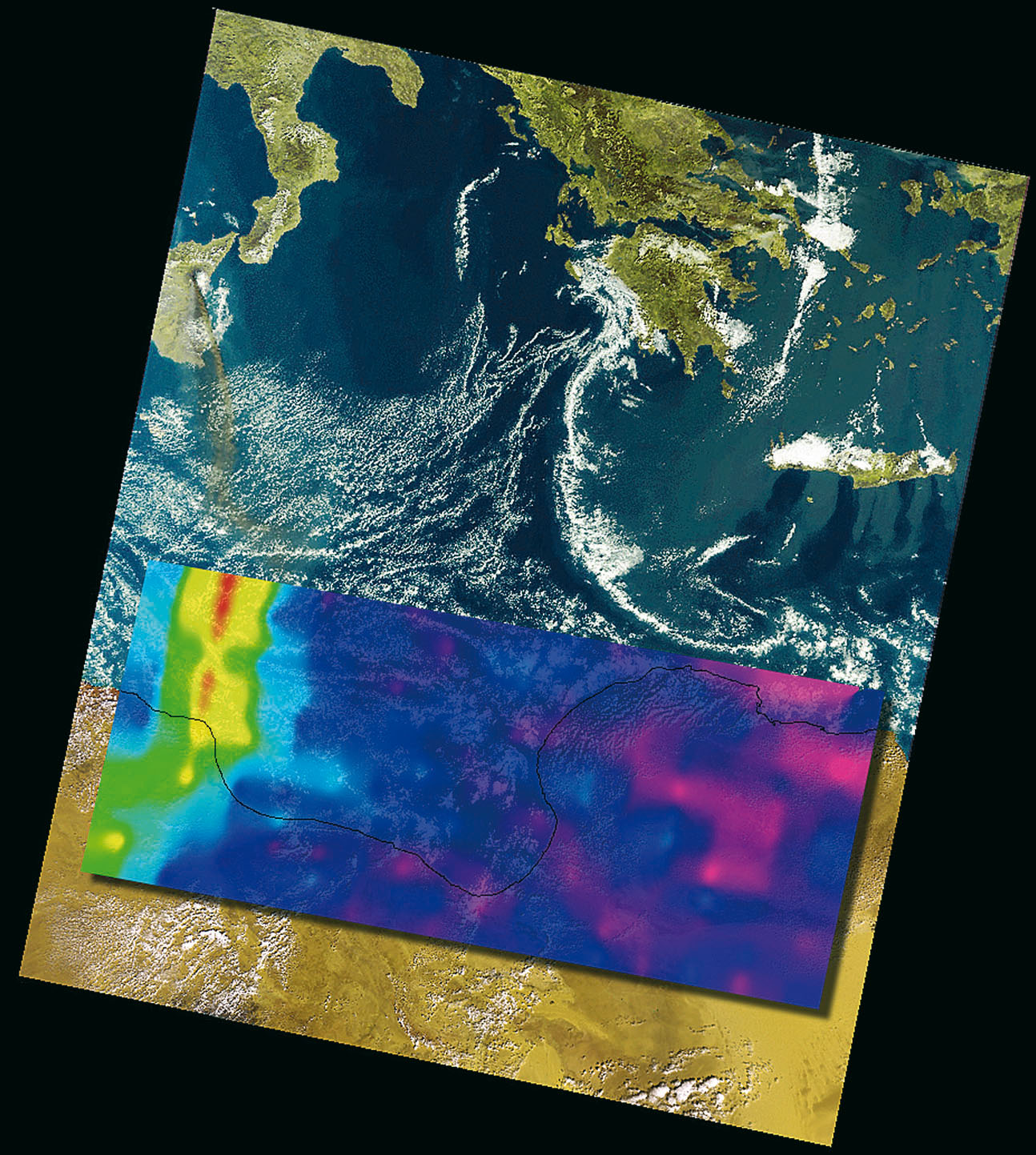
| Fig. 10-12 |
The Mt. Etna volcanic eruption in 2002 with obvious SO2 emissions (reddish plume). The SCIAMACHY nadir measurement
is overlayed on a MERIS image showing that the plume of SO2 and the visible ash cloud match well.
(Courtesy: ESA and Brockmann Consult) |
|
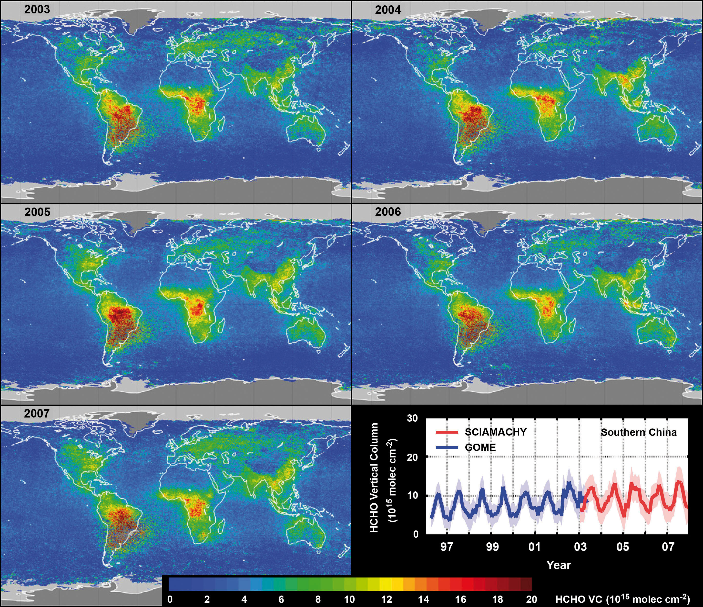
| Fig. 10-13 |
Yearly averaged SCIAMACHY HCHO vertical columns from 2003-2007. The HCHO trend over China is indicated in the bottom right panel,.
(Courtesy: adapted from De Smedt et al. 2008) |
|
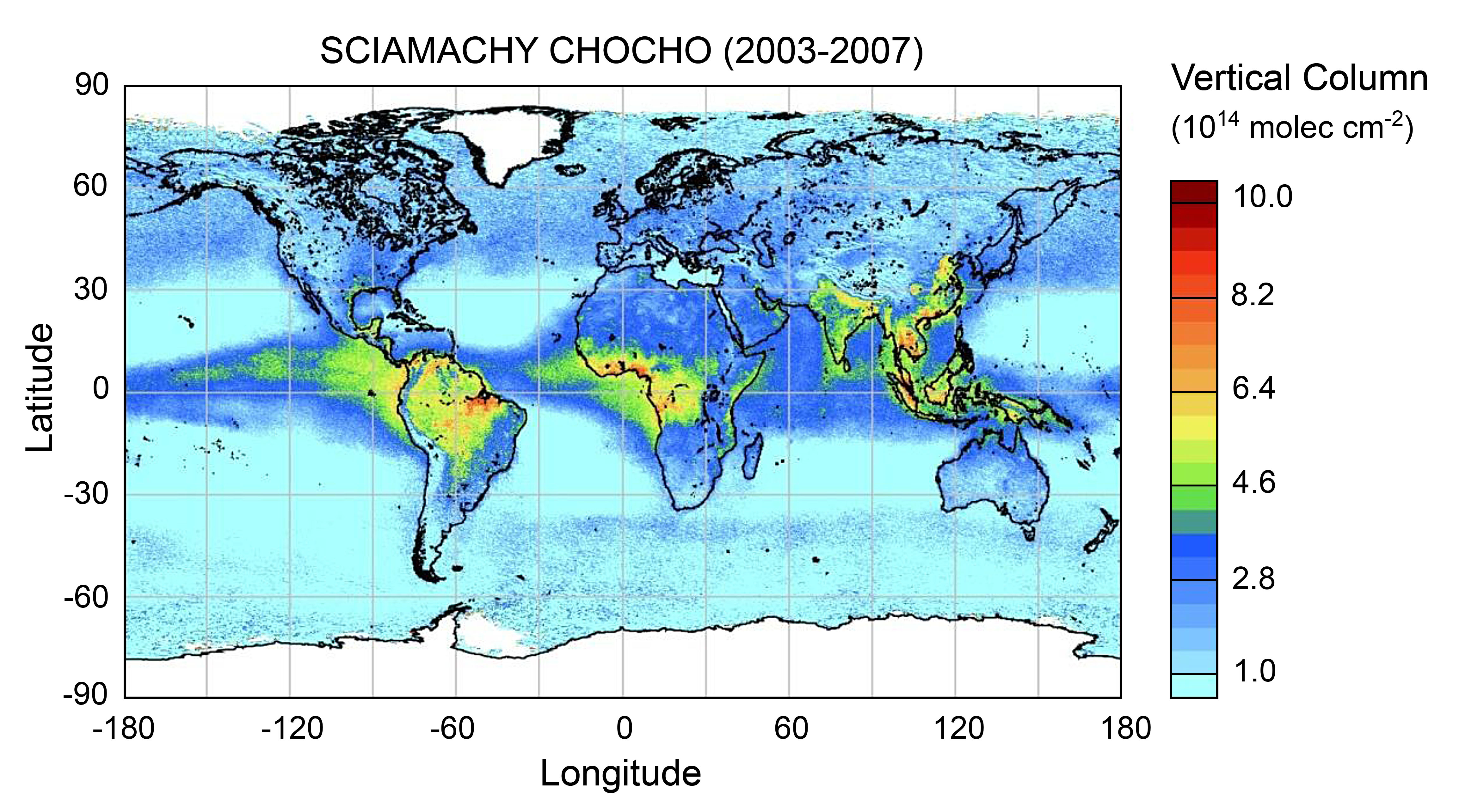
| Fig. 10-14 |
Multiannual (2003-2007) SCIAMACHY CHOCHO vertical columns. The largest amounts are found over the tropics and
sub-tropics where vegetation and biomass burning is abundant. (Courtesy: Vrekoussis et al. 2009) |
|
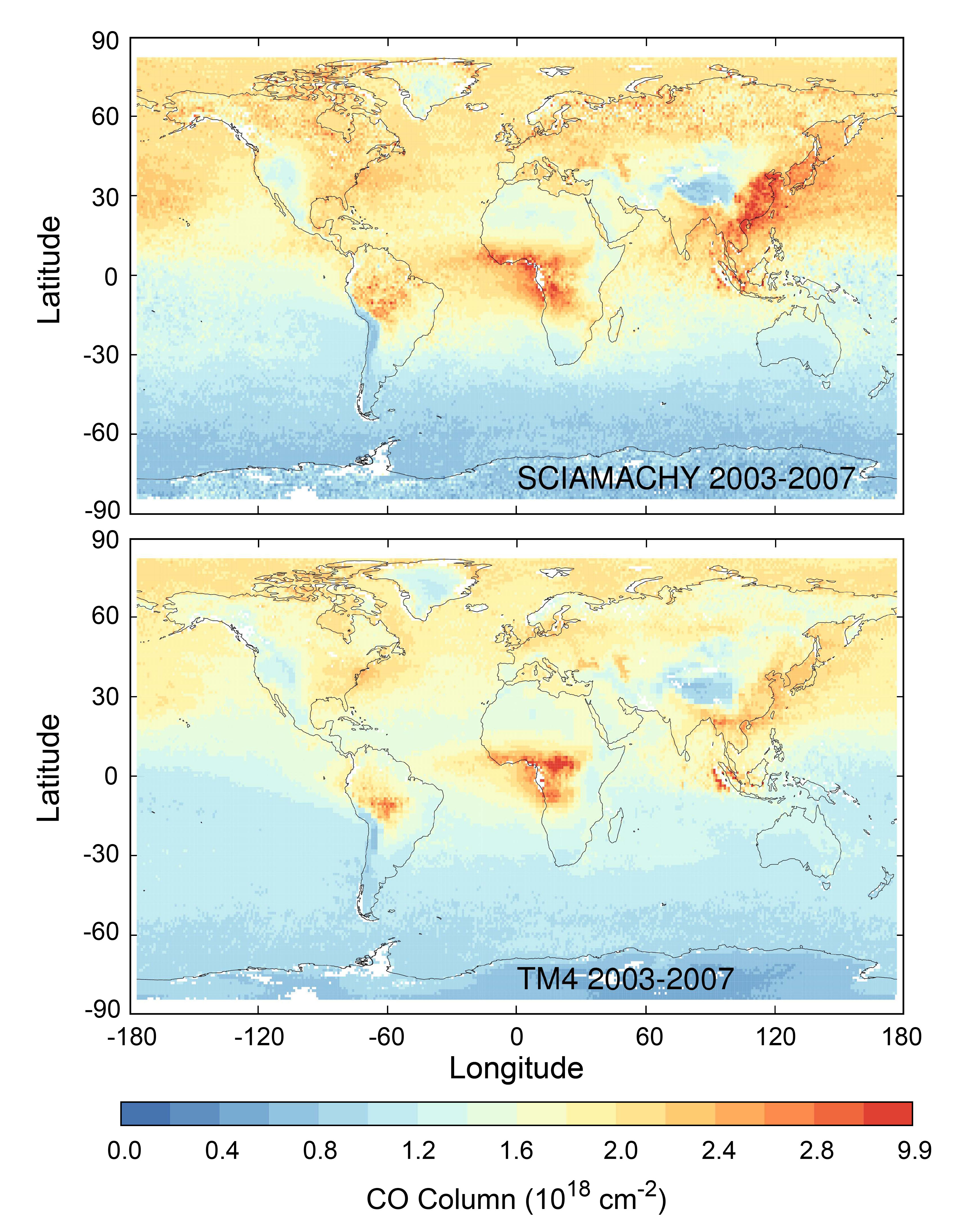
| Fig. 10-15 |
Five year (2003-2007) average CO total columns on a 1° ´ 1° grid as retrieved by SCIAMACHY (top) and the TM4
chemistry-transport model (bottom). The SCIAMACHY CO columns above low clouds over sea are filled up with TM4
CO densities below the cloud to obtain total columns (Courtesy: Gloudemans et al. 2009) |
|
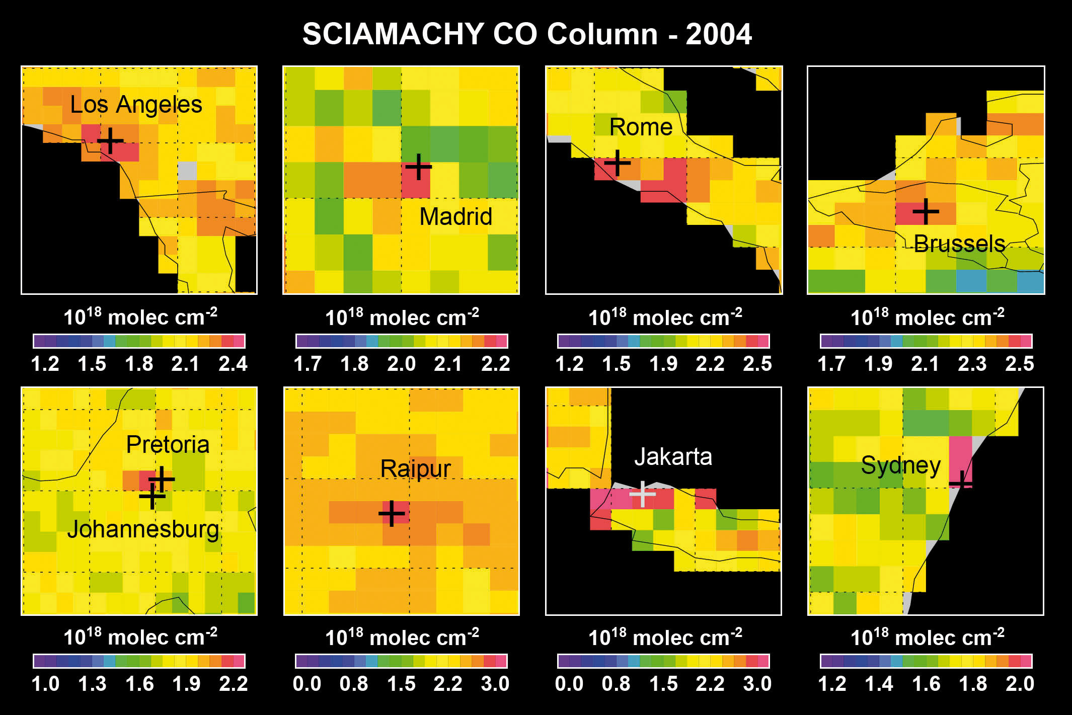
| Fig. 10-16 |
A variety of urban areas as detected in SCIAMACHY CO data in 2004.
(Courtesy: M. Buchwitz, IUP-IFE, University of Bremen) |
|
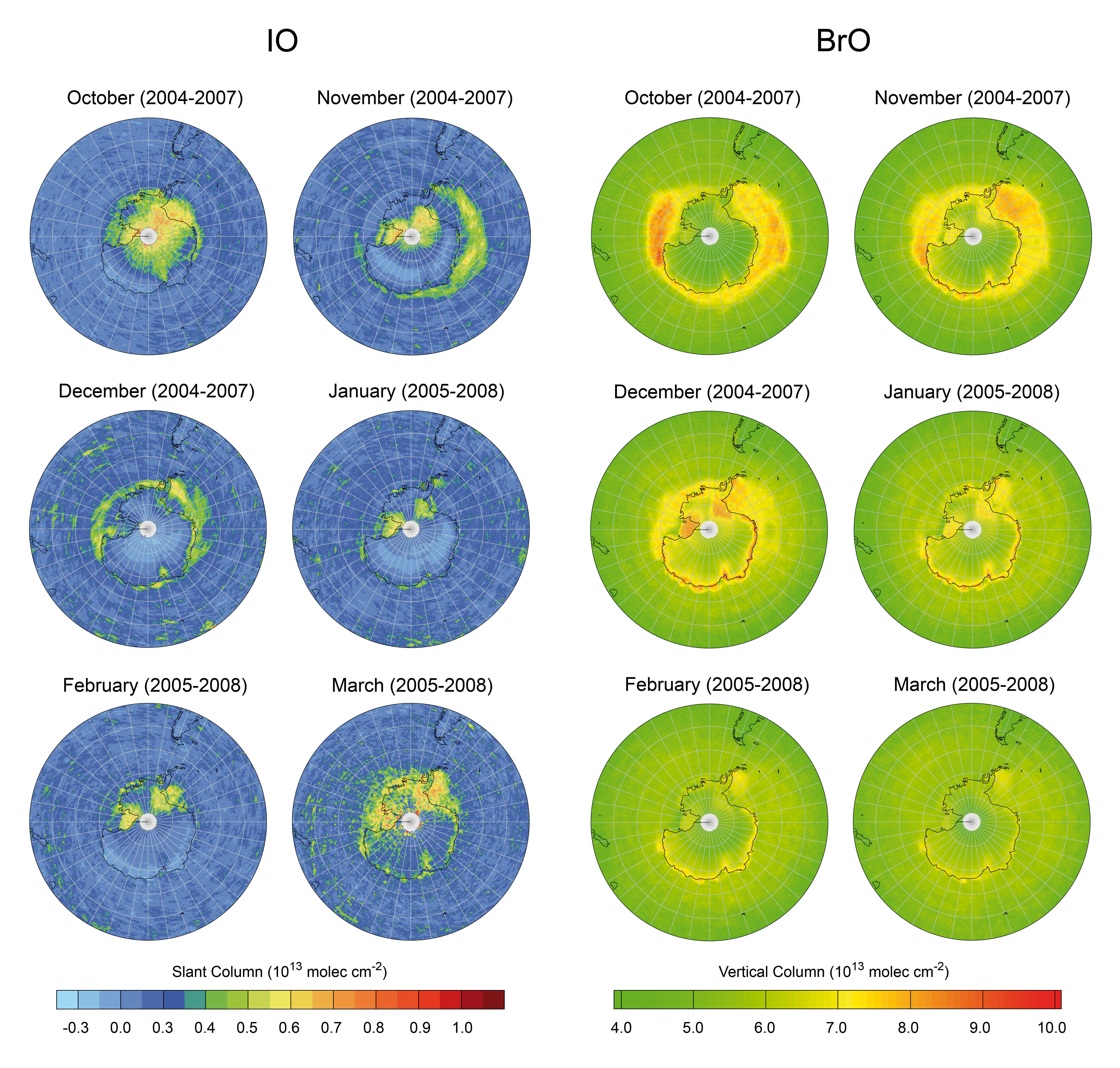
| Fig. 10-17 |
Monthly maps of SCIAMACHY observations of IO (left) and BrO (right), averaged over four subsequent years from 2004-2008.
A stratospheric air mass factor (AMF) is applied to the BrO columns only, leaving the patterns of IO and BrO still comparable.
Courtesy: A. Schönhardt, IUP-IFE, University of Bremen) |
|
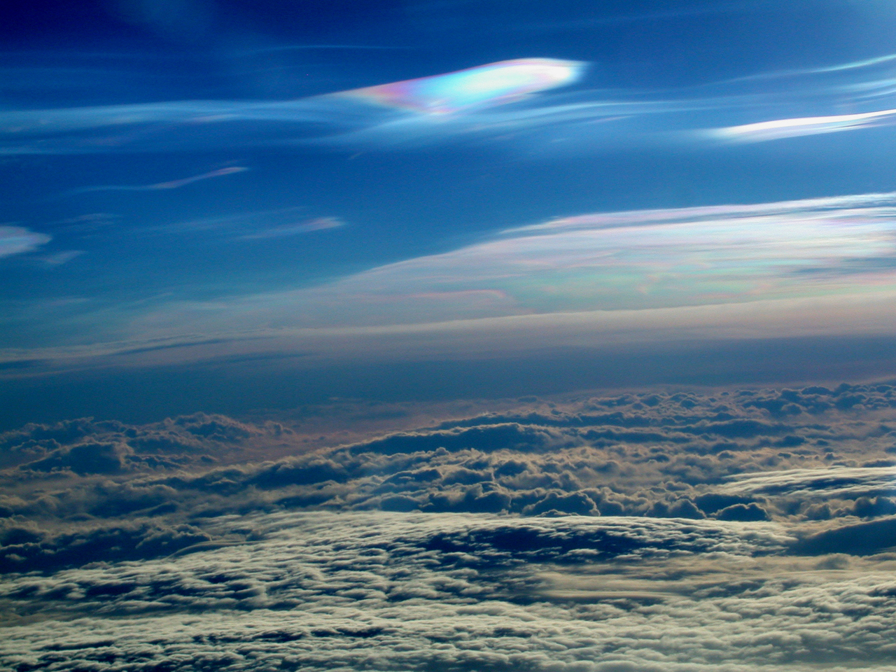
| Fig. 10-18 |
Polar Stratospheric Clouds over Southern Norway in January 2003, taken from the NASA DC-8 aircraft at an altitude
of 11 km. The PSC hover well above the tropospheric cloud cover. (Photo: P. Newman, NASA/GSFC) |
|
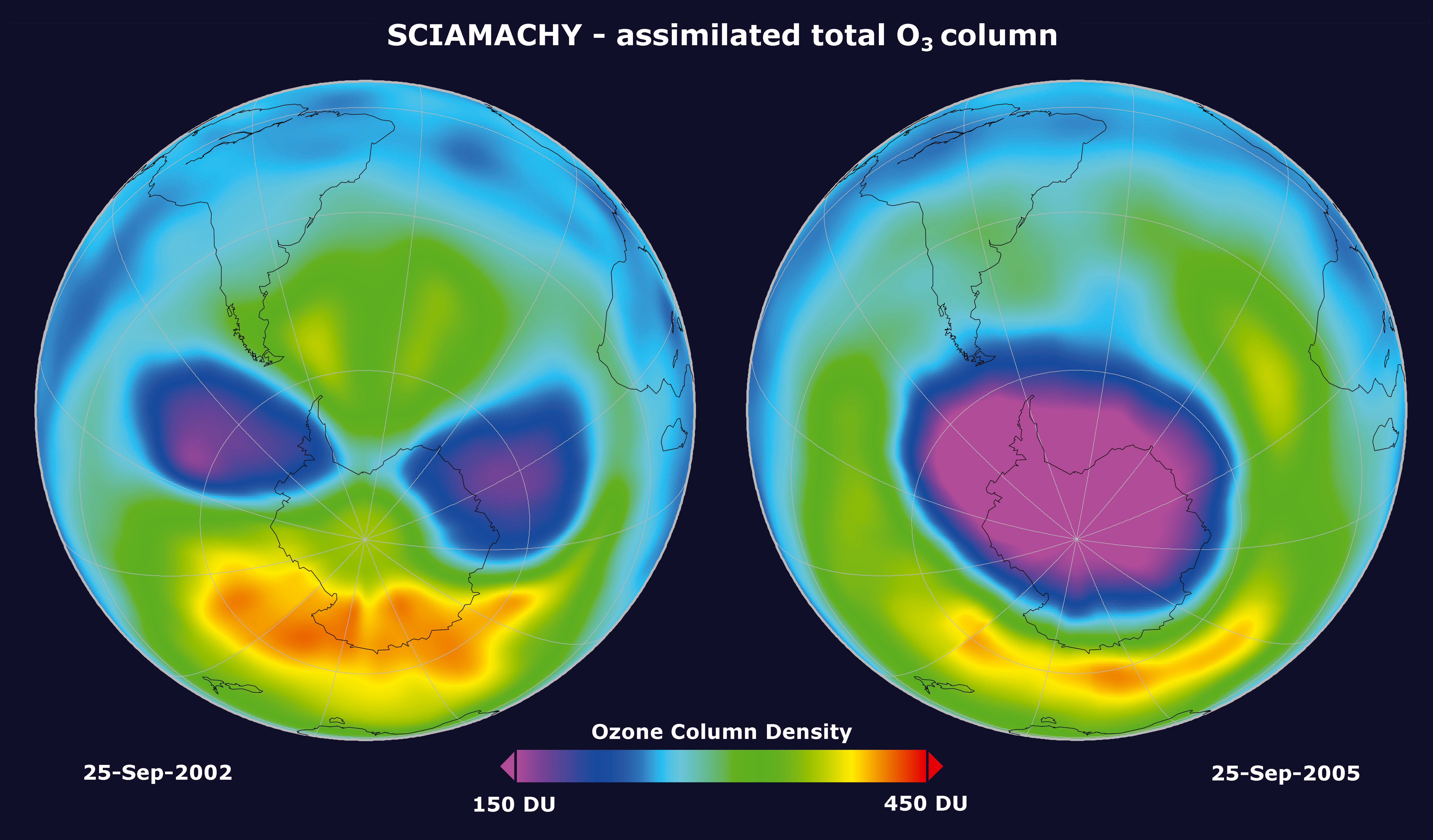
| Fig. 10-19 |
The Antarctic ozone hole in 2002 (left) and 2005 (right). SCIAMACHY total column ozone measurements from 25 September
have been analysed with the ROSE assimilation model to generate this view. Due to meteorological conditions, the hole
as split and reduced in size in 2002 but appeared 'as normal' in 2005. (Courtesy: T. Erbertseder, DLR-DFD) |
|
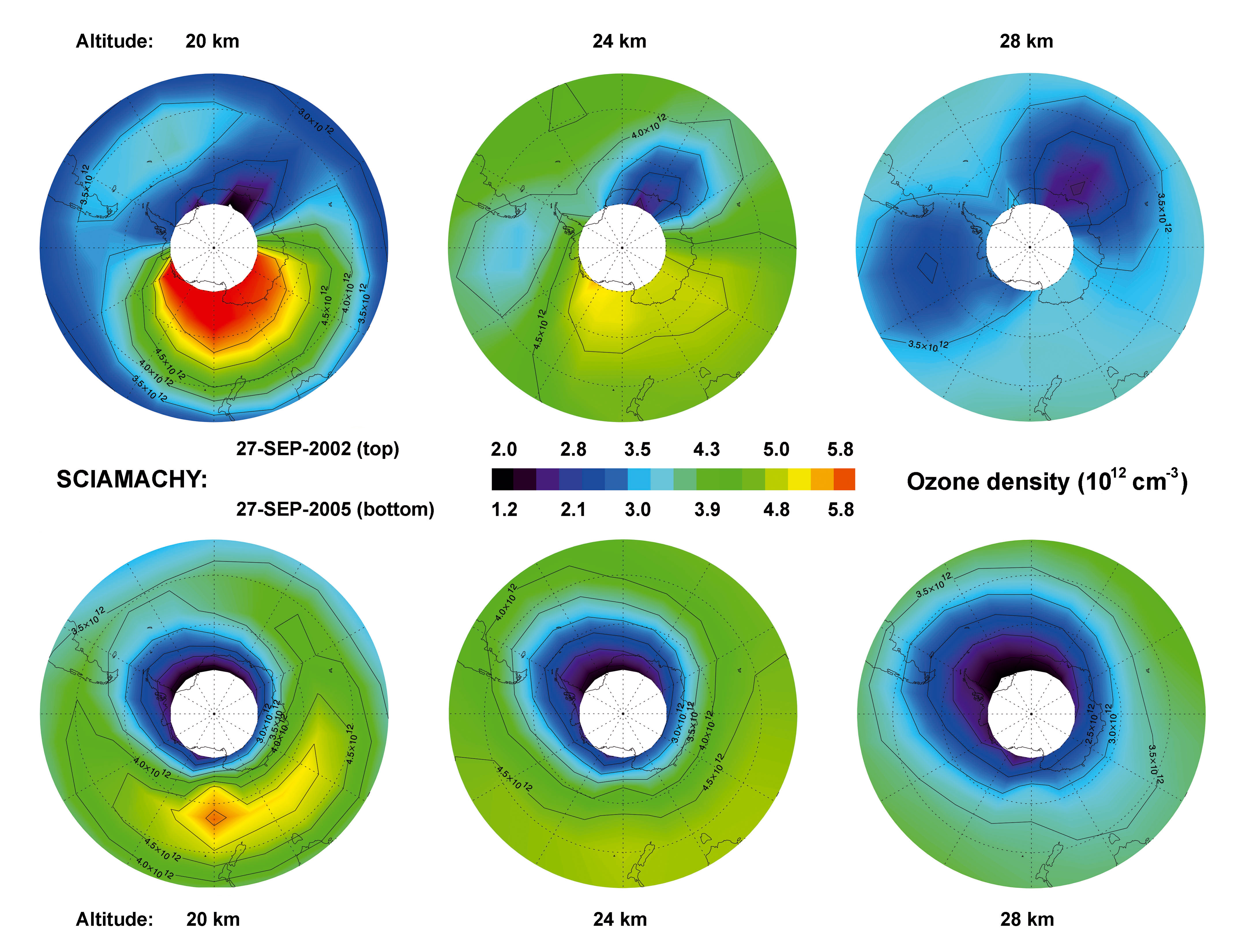
| Fig. 10-20 |
Slices of the polar southern hemisphere ozone field at altitudes of approximately 20, 24 and 28 km on 27 September 2002
and 27 September 2005 as measured by SCIAMACHY. The observed split of the ozone hole in 2002 is not so obvious in the
lower stratosphere around 20 km, but clearly visible at 24 and 28 km. In 2005, an ozone hole of 'normal shape' existed
at all altitudes. (Courtesy: C. von Savigny, IUP-IFE, University of Bremen) |
|
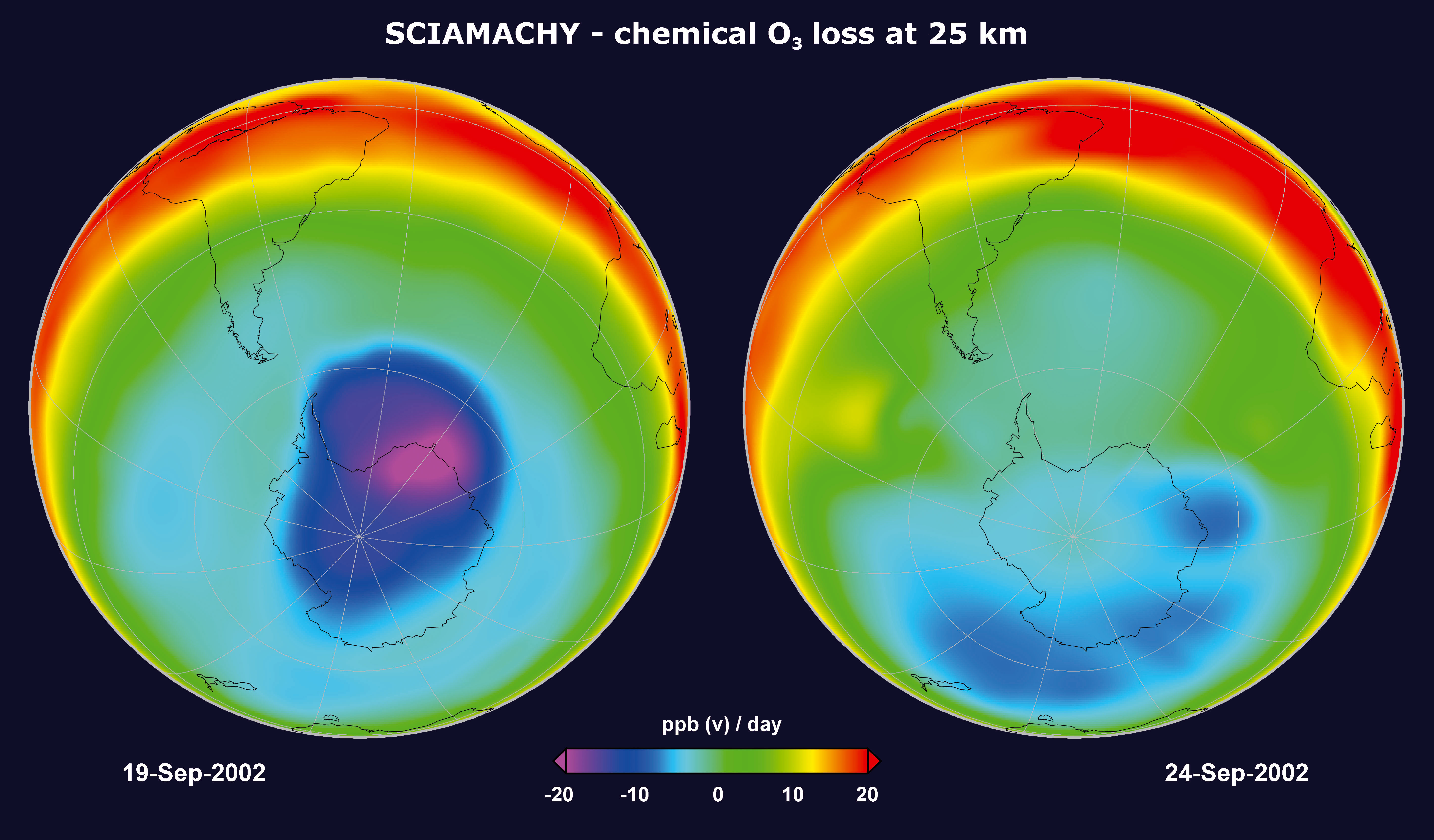
| Fig. 10-21 |
Chemical ozone loss rates on two days in September 2002 in the mid-stratosphere at about 25 km, relative to the previous day.
While on 19 September the ozone hole was still developing its usual shape, 5 days later the split-up of the vortex has reduced
ozone loss rates. (Courtesy: T. Erbertseder, DLR-DFD) |
|
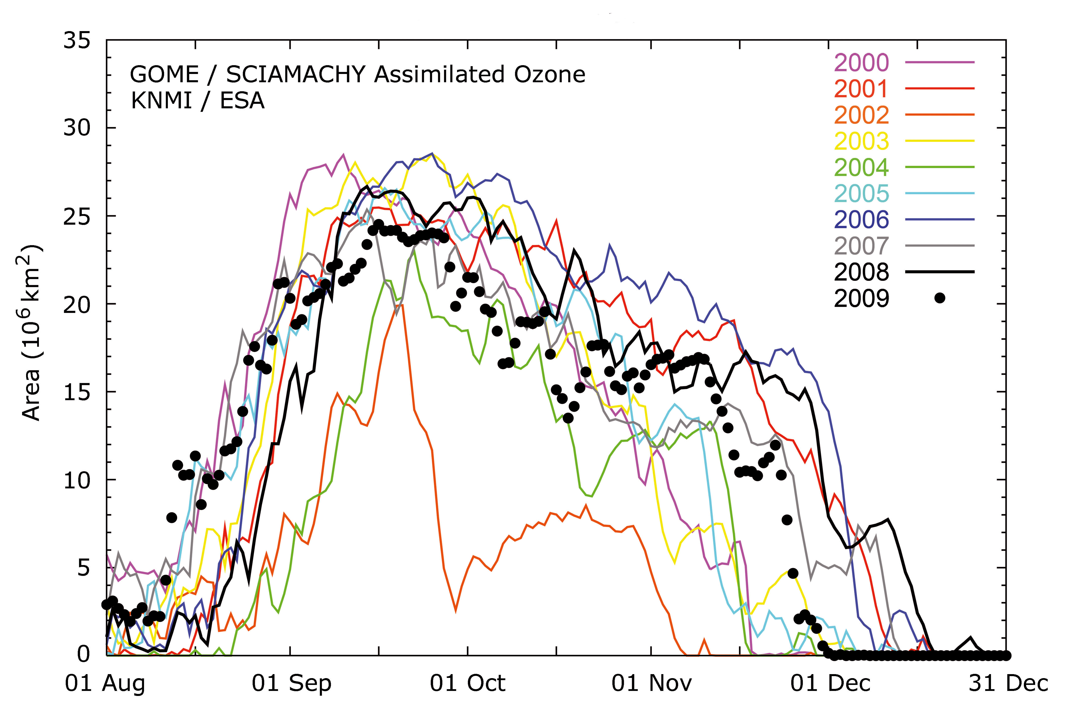
| Fig. 10-22 |
Time series of the size of the Antarctic ozone hole from 2000-2009 based on observations of GOME and SCIAMACHY. The area
includes ozone column values below 30°S lower than 220 Dobson Units. (Courtesy: TEMIS KNMI/ESA) |
|
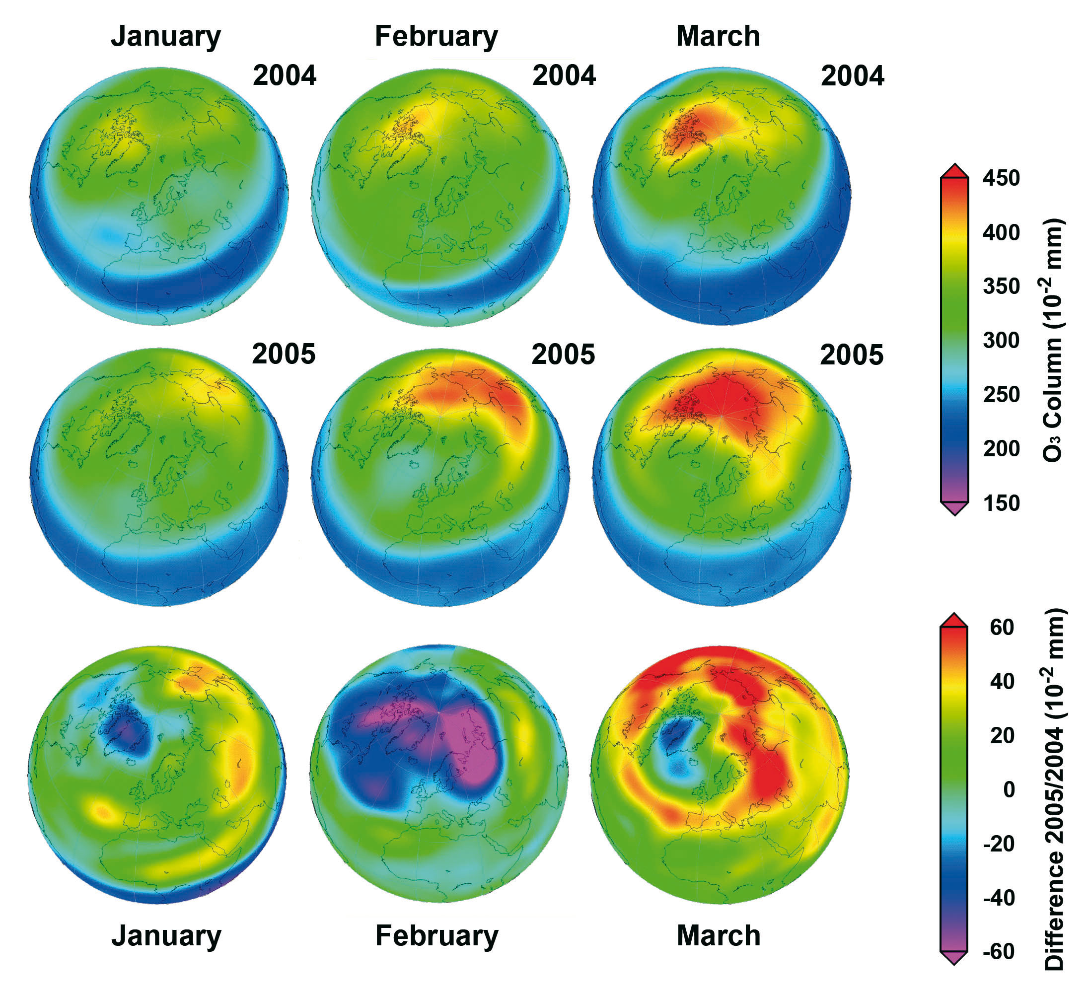
| Fig. 10-23 |
Ozone columns over the northern hemisphere for late winter/early spring 2004 (top row), 2005 (mid row) and the
difference between both years (bottom row). Owing to unusual low temperatures in the stratosphere over the Arctic,
significant ozone loss occurred in February 2005 with a recovery of the ozone layer in March.
(Courtesy: J. Meyer-Arnek, DLR-DFD) |
|
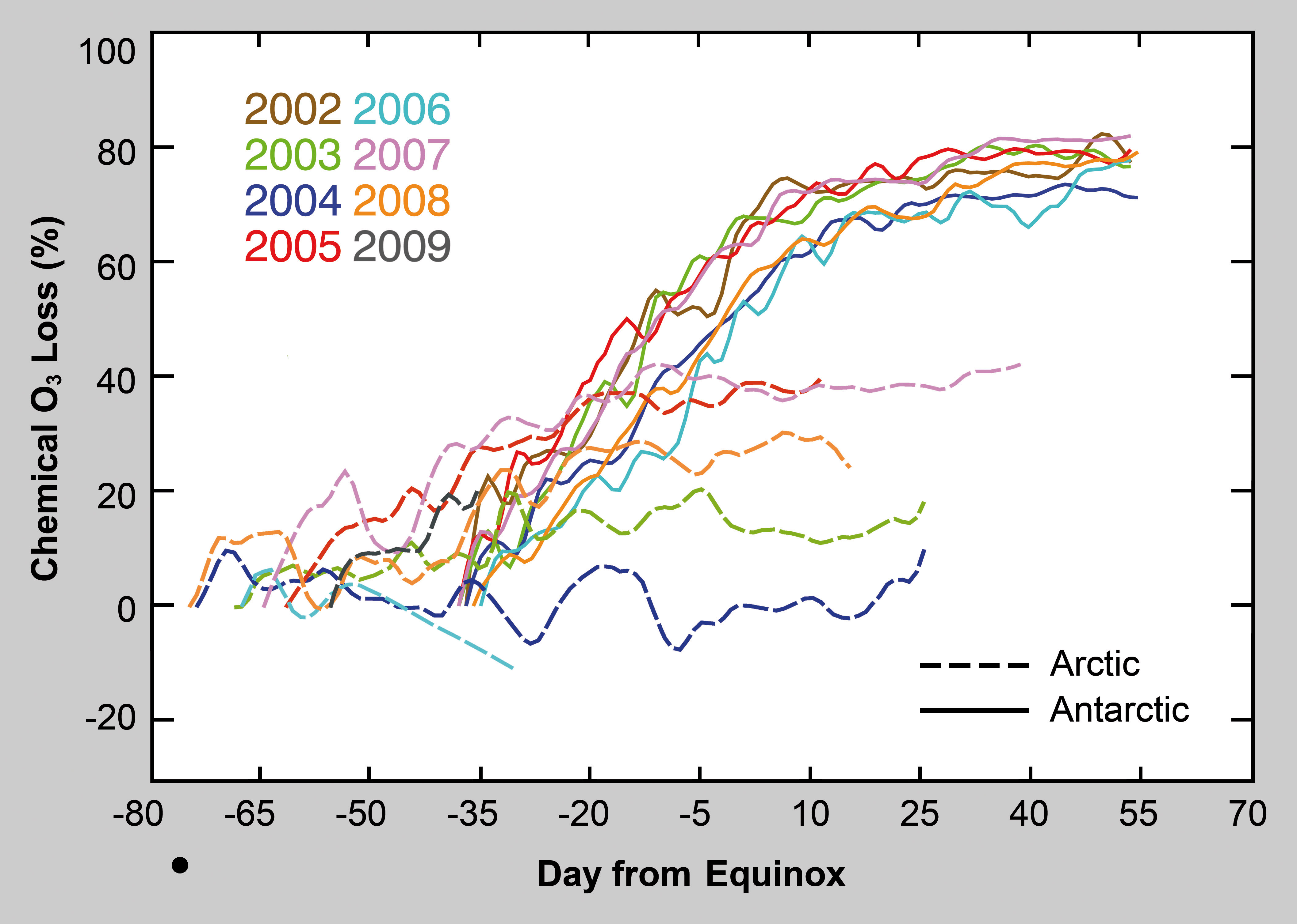
| Fig. 10-24 |
Relative chemical ozone losses at the 475 K isentropic level (around 18 km) for the period 2002-2009 in the Arctic
(dotted lines) and Antarctic (solid lines) polar vortices. (Courtesy: IUP-IFE, University of Bremen) |
|
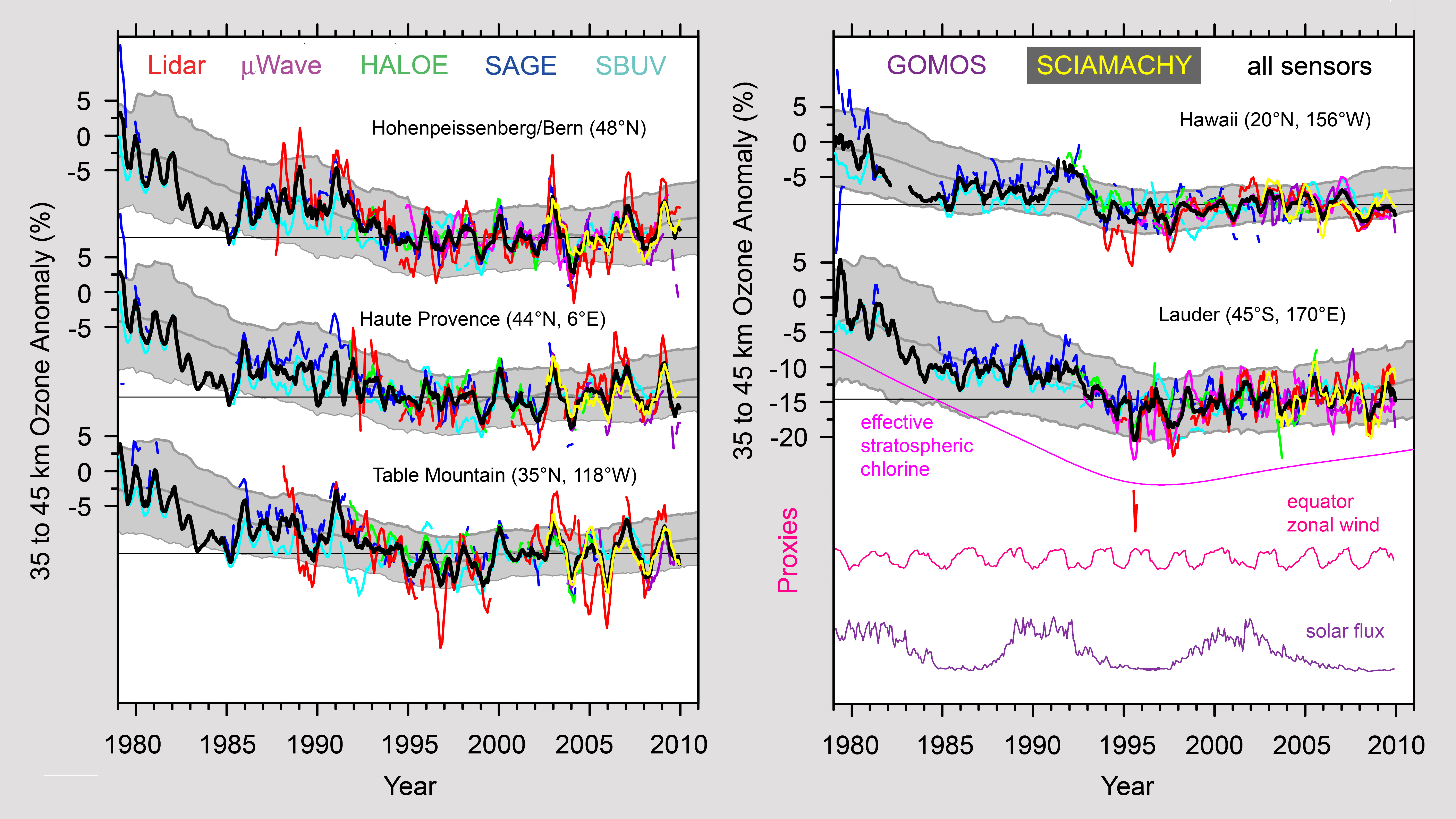
| Fig. 10-25 |
Ozone anomalies from 1979 to 2009 derived from different datasets at five NDACC stations. The anomalies are averaged over the
35-45 km range. The all-instrument average is shown in black. All time series were smoothed by a 5-month running mean. At the
bottom of the right hand panel 3 proxies are given: The negative 10 hPa zonal wind at the equator for the QBO, the 10.7 cm solar
flux for the 11-year solar cycle and the inverted effective stratospheric chlorine for ozone destruction by chlorine. The grey
line and the grey shaded area show model simulations and their 2-sigma standard deviation.
(Courtesy: adapted from Steinbrecht et al. 2009, reproduced/modified by permission of American Geophysical Union) |
|
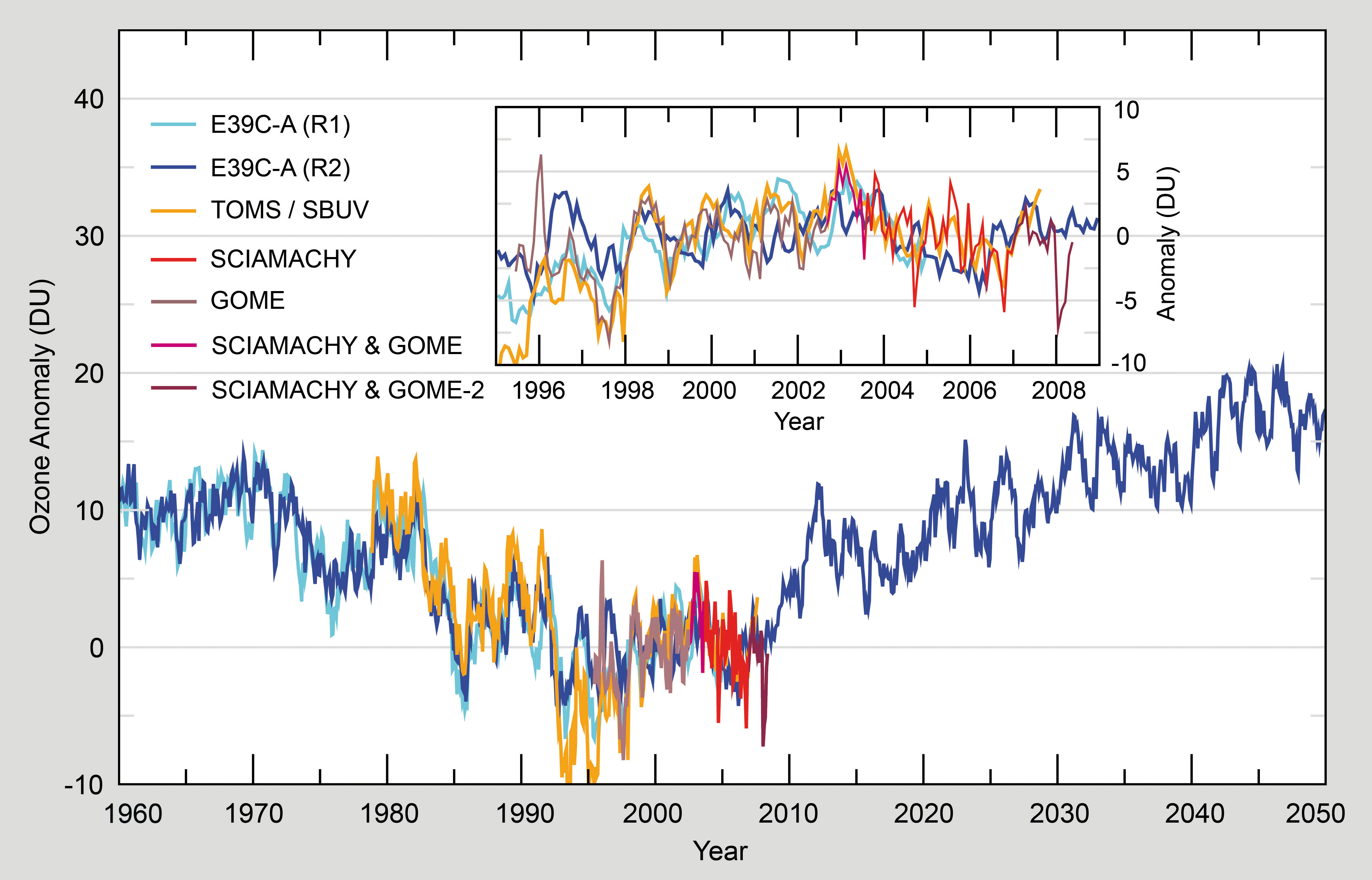
| Fig. 10-26 |
Total ozone anomaly from 60°N to 60°S from the merged GOME/SCIAMACHY/GOME-2 dataset. For comparison, the
results from the merged TOMS/SBUV/OMI are given, together with predictions from climate-chemistry model runs.
(Courtesy: Loyola et al. 2009, reproduced/modified by permission of American Geophysical Union) |
|
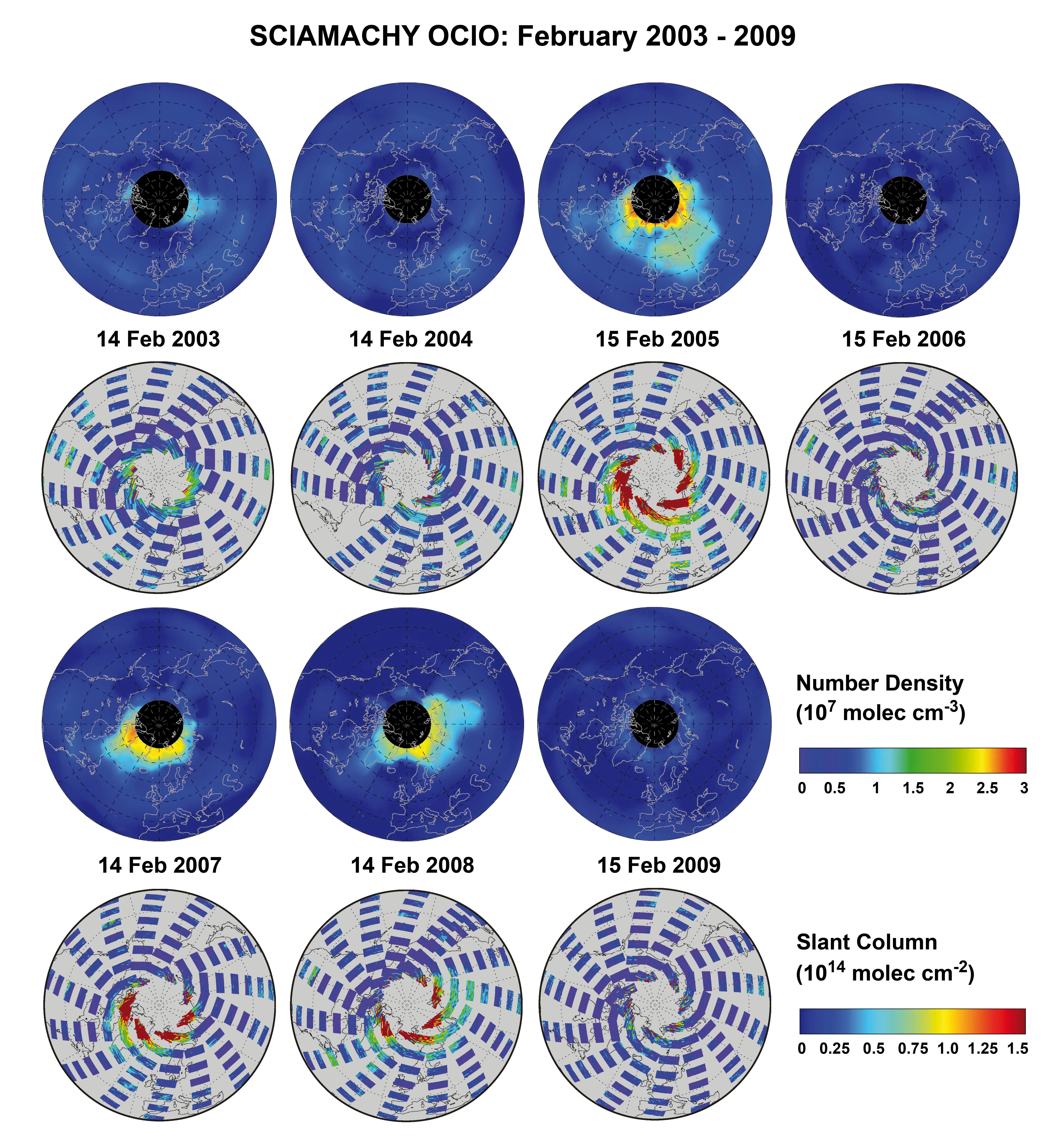
| Fig. 10-27 |
OClO number density at 19 km altitude above the northern hemisphere derived from SCIAMACHY limb observations
(rows 1 and 3), and the corresponding total OClO slant column derived from nadir views (rows 2 and 4) for mid of February
in the Arctic winters 2002/03 to 2008/09. (Courtesy: S. Kühl; MPI for Chemistry, Mainz) |
|
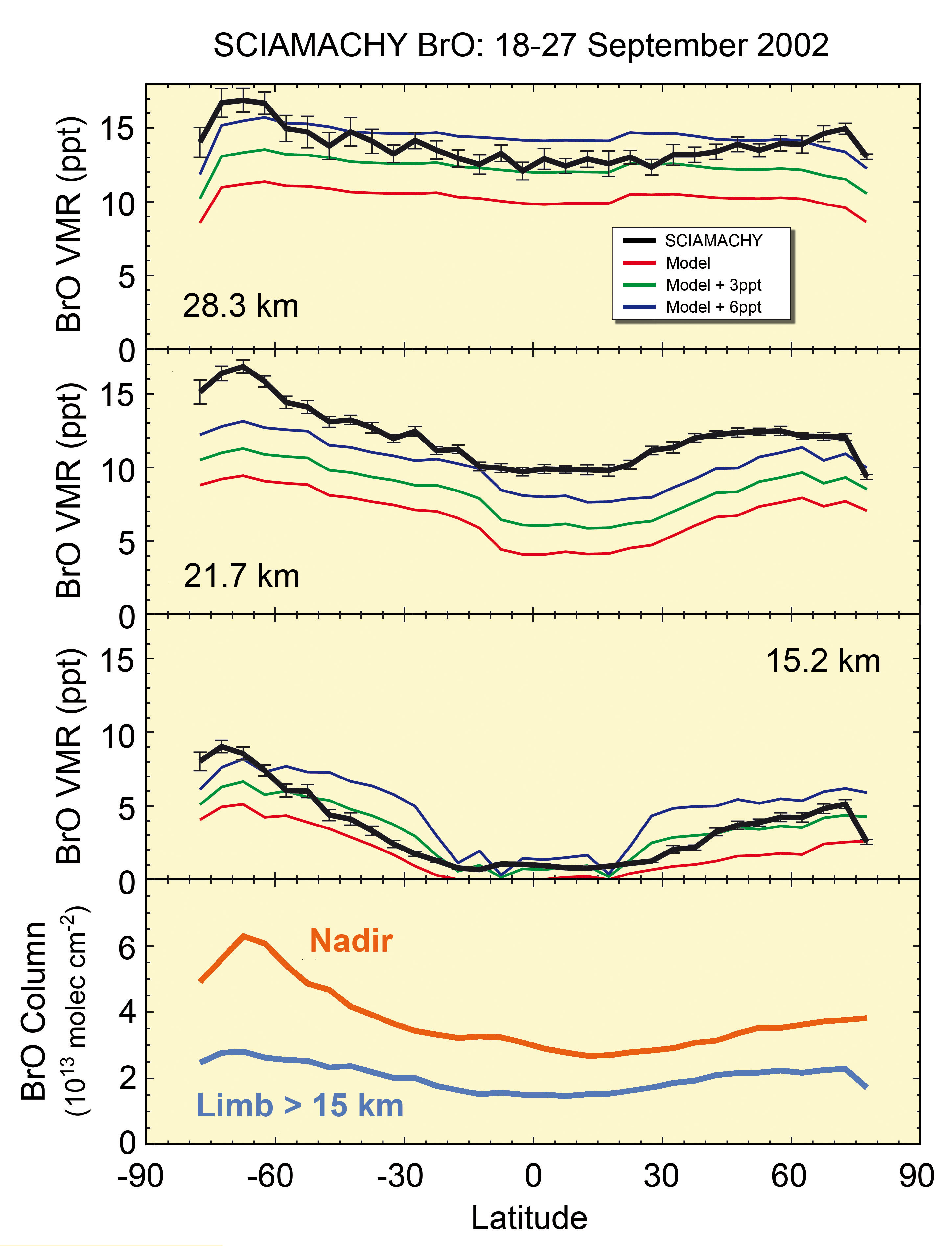
| Fig. 10-28 |
Zonal mean BrO at selected altitudes obtained from SCIAMACHY limb observations and from model calculations.
Additional bromine of 0, 3, and 6 pptv, respectively, has been added to the model calculations to account for the
contribution from very short-lived substances (VSLS). (Courtesy: adapted from WMO 2007 - based on Sinnhuber et al. 2005) |
|
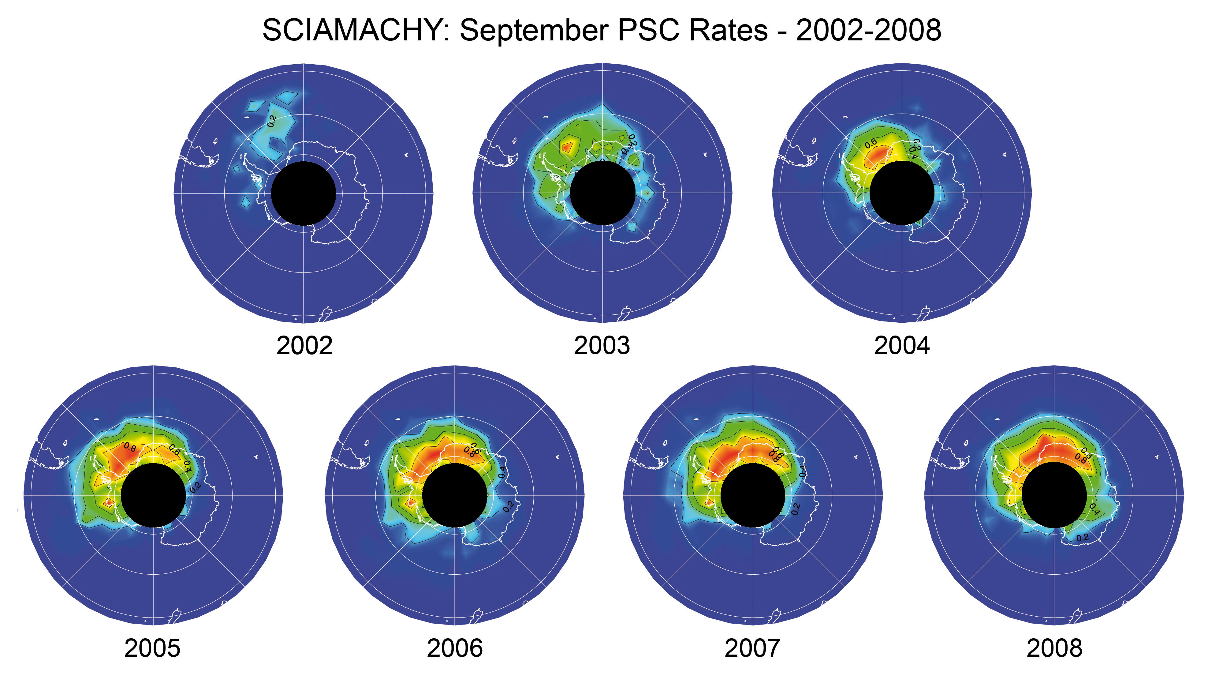
| Fig. 10-29 |
Maps of PSC occurrence rates for September of the years 2002-2008. Contours levels correspond to 0.2, 0.4, 0.6, and 0.8.
Red areas indicate occurrence rates exceeding 0.8. (Courtesy: C. von Savigny, IUP-IFE, University of Bremen) |
|
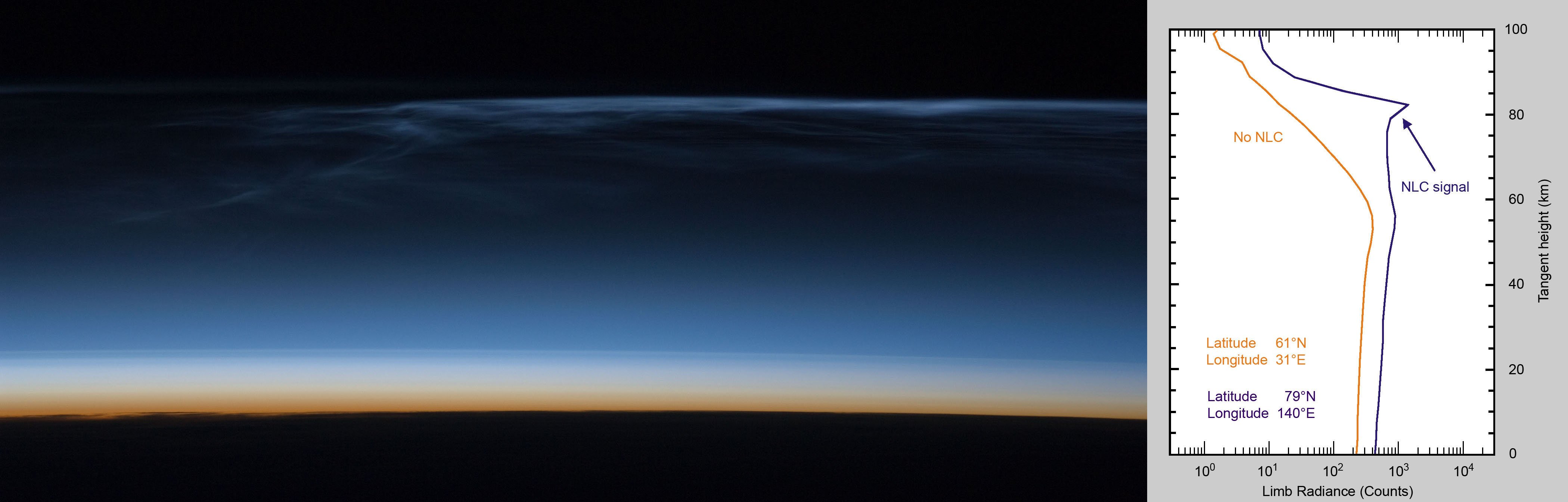
| Fig. 10-30 |
NLC as seen from the International Space Station on 22 July 2008 (left panel), together with the NLC
signature in a SCIAMACHY UV limb radiance profile from 3 July 2002 (right panel). The scattering by ice particles
in the NLC leads to a significant increase of the observed limb radiance profile peaking at the characteristic NLC
altitude of about 83-85 km (blue line). For comparison, a limb radiance measurement in the absence of NLC is shown
in red. (Courtesy: C. von Savigny, IUP-IFE, University of Bremen; ISS photo: NASA) |
|
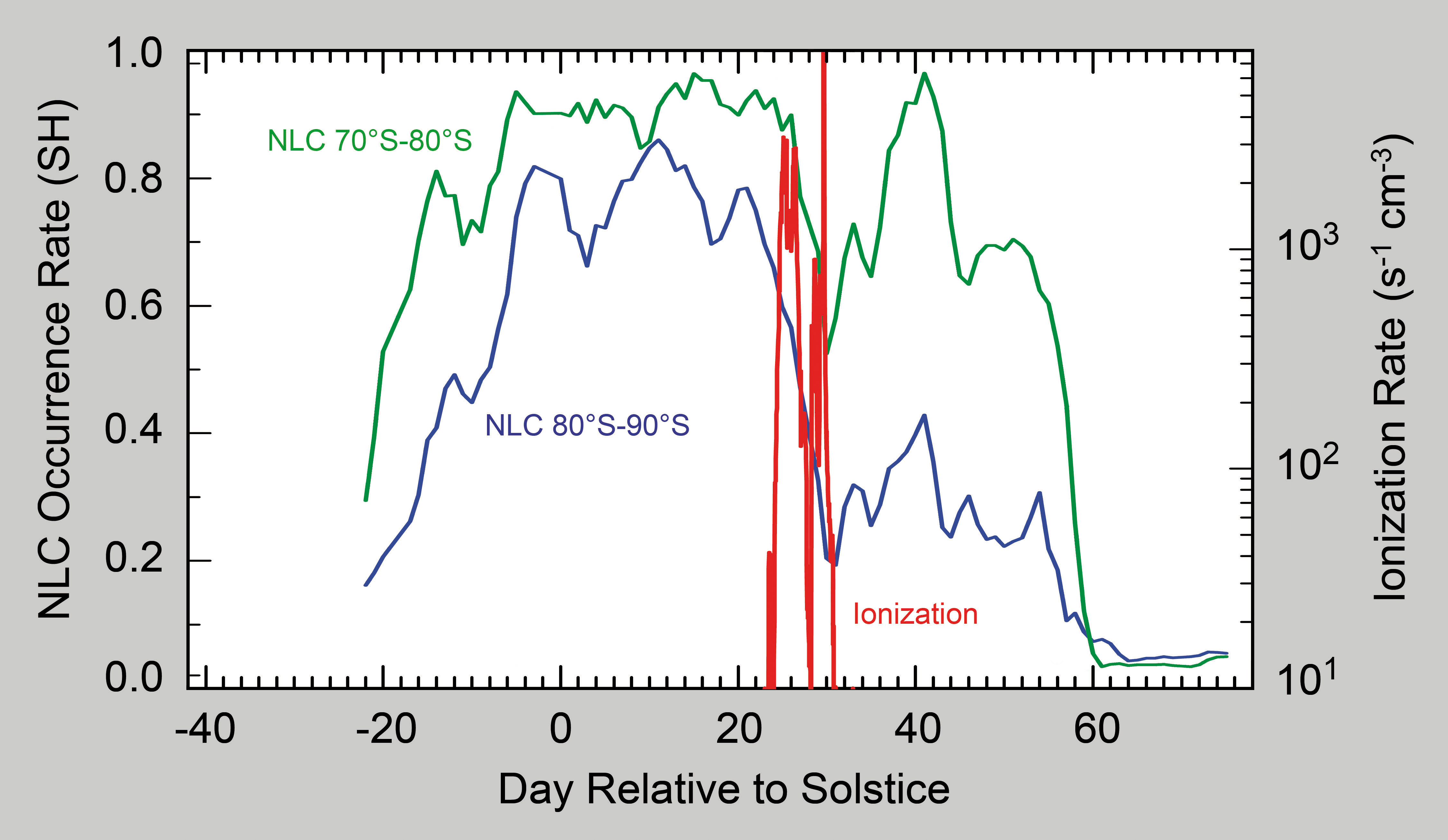
| Fig. 10-31 |
Smoothed zonally averaged NLC occurrence rates in the southern hemisphere NLC season 2004/2005 (left abscissa)
and ionisation rates at 82 km (right abscissa). At the time of the solar proton event, the ionisation rate
increases and causes a drop in the NLC rate. (Courtesy: C. von Savigny, IUP-IFE, University of Bremen) |
|
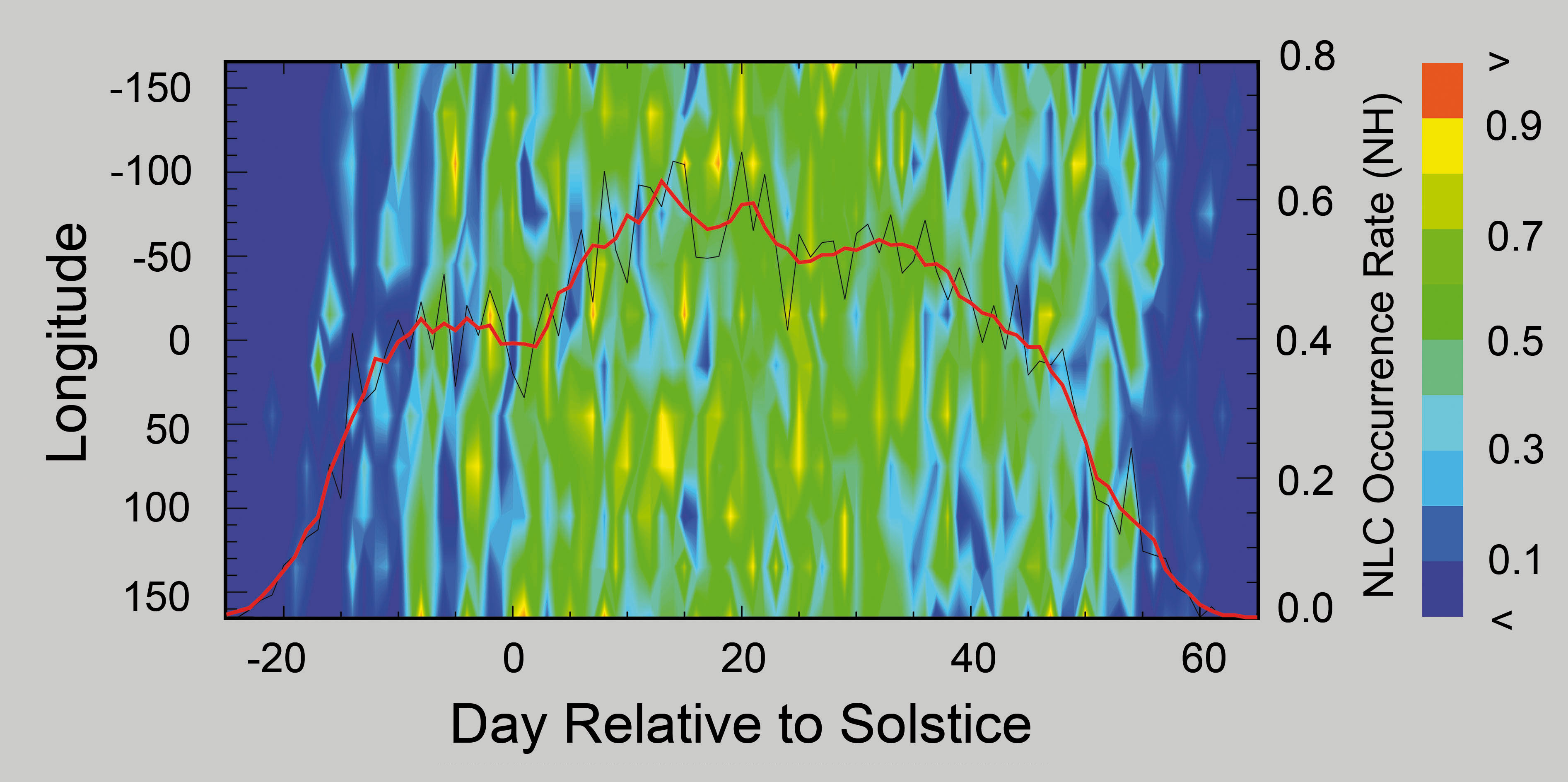
| Fig. 10-32 |
Contour plot of the longitude and time dependence of the NLC occurrence rate for 2005 in the northern hemisphere
with the zonally averaged NLC occurrence rate overlaid (red curve, right abscissa). The 5-day wave pattern is
clearly visible at the beginning of the NLC season as a westward propagating signature with wavenumber 1 and a
period of 5 days. (Courtesy: C. von Savigny, IUP-IFE, University of Bremen) |
|
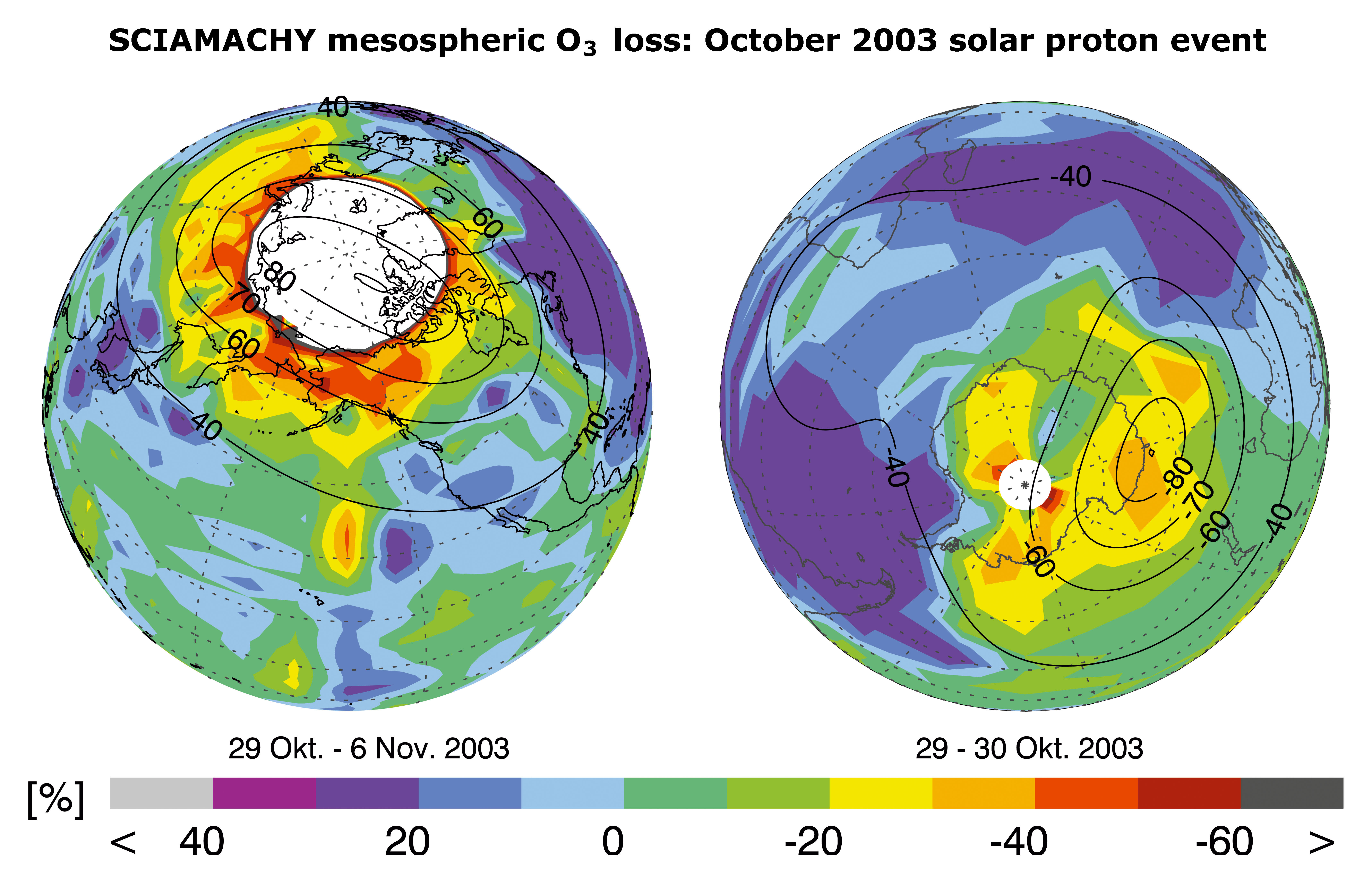
| Fig. 10-33 |
Measured change of ozone concentration at 49 km altitude due to the strong solar proton events end of
October 2003 in the northern and southern hemisphere relative to the reference period of 20-24 October 2003.
White areas depict regions with no observations. The black solid lines are the Earth's magnetic latitudes at
60 km altitude for 2003. (Courtesy: Rohen et al. 2005) |
|
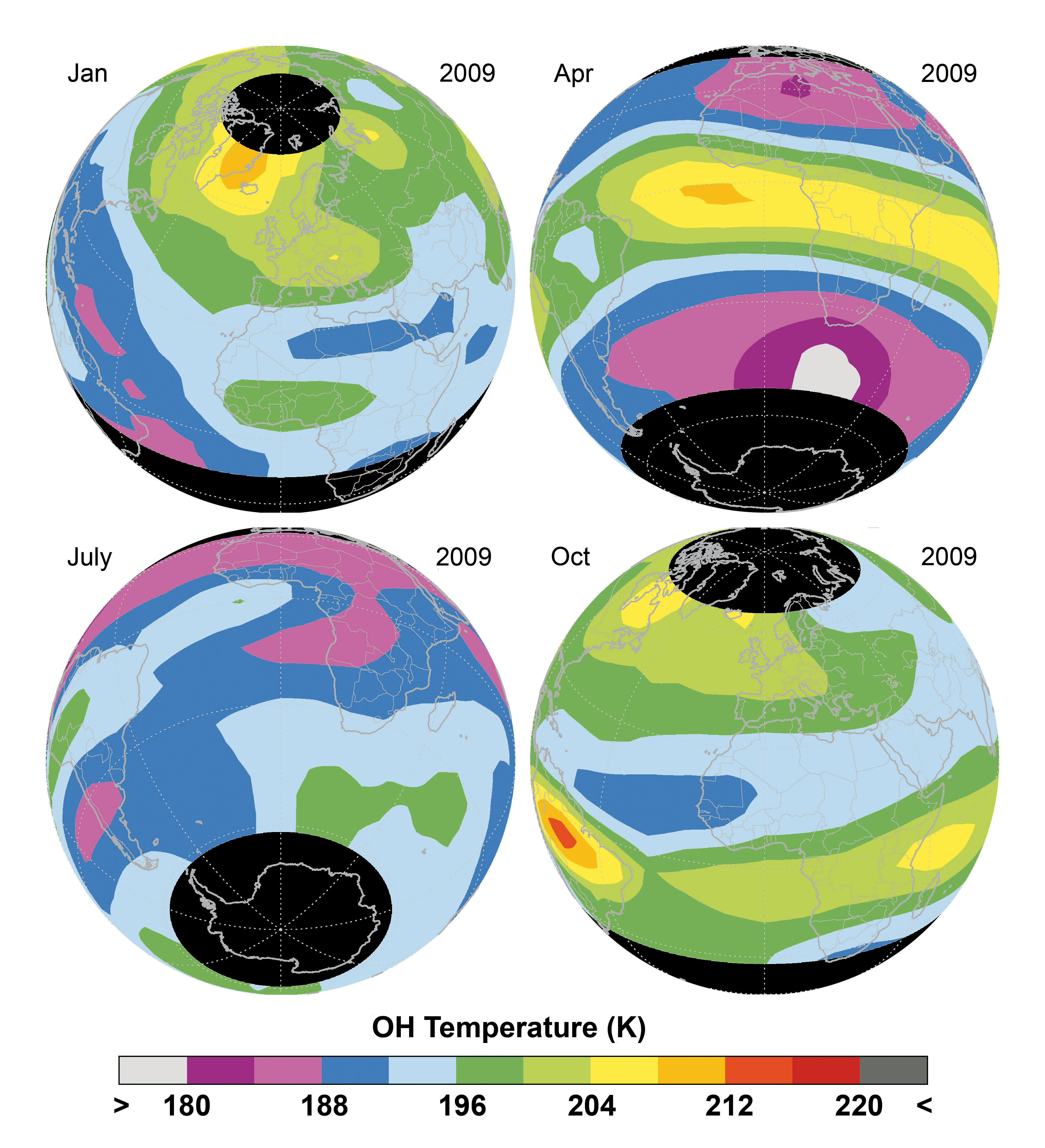
| Fig. 10-34 |
Monthly averaged SCIAMACHY retrievals of OH rotational temperatures at about 87 km for
January, April, July and October 2009. (Courtesy: K.-U. Eichmann, IUP-IFE, University of Bremen) |
|
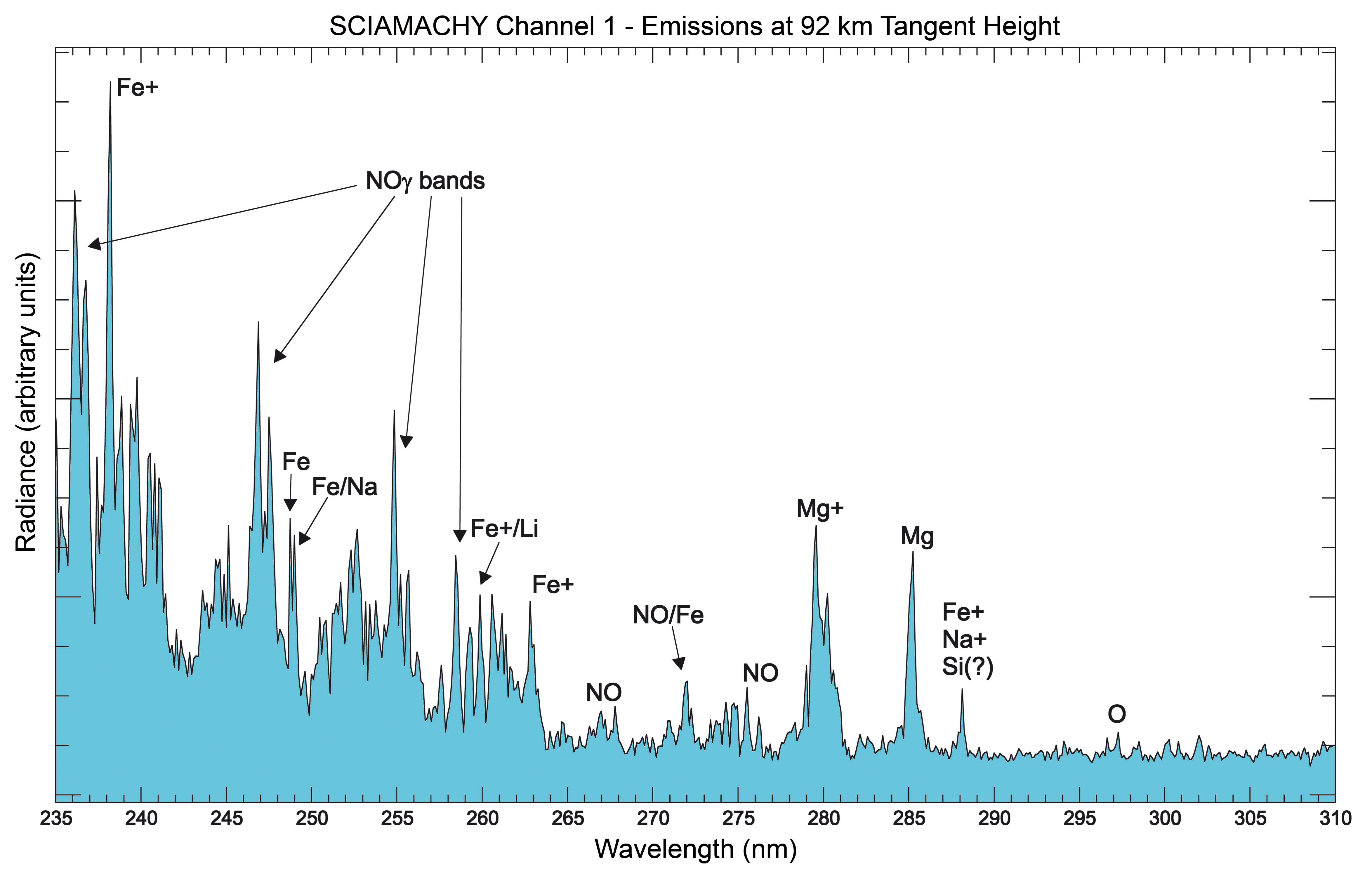
| Fig. 10-35 |
Emission lines in SCIAMACHY limb radiance in channel 1 at the highest limb tangent altitude,
normalised to the solar irradiance, in arbitrary units. A number of emission signals are detected.
The most dominant features are the NO gamma-bands and MgII, but signals from neutral Mg, atomic oxygen,
Si, Fe and Fe+ are observed, as well. (Courtesy: M. Sinnhuber, IUP-IFE, University of Bremen) |
|
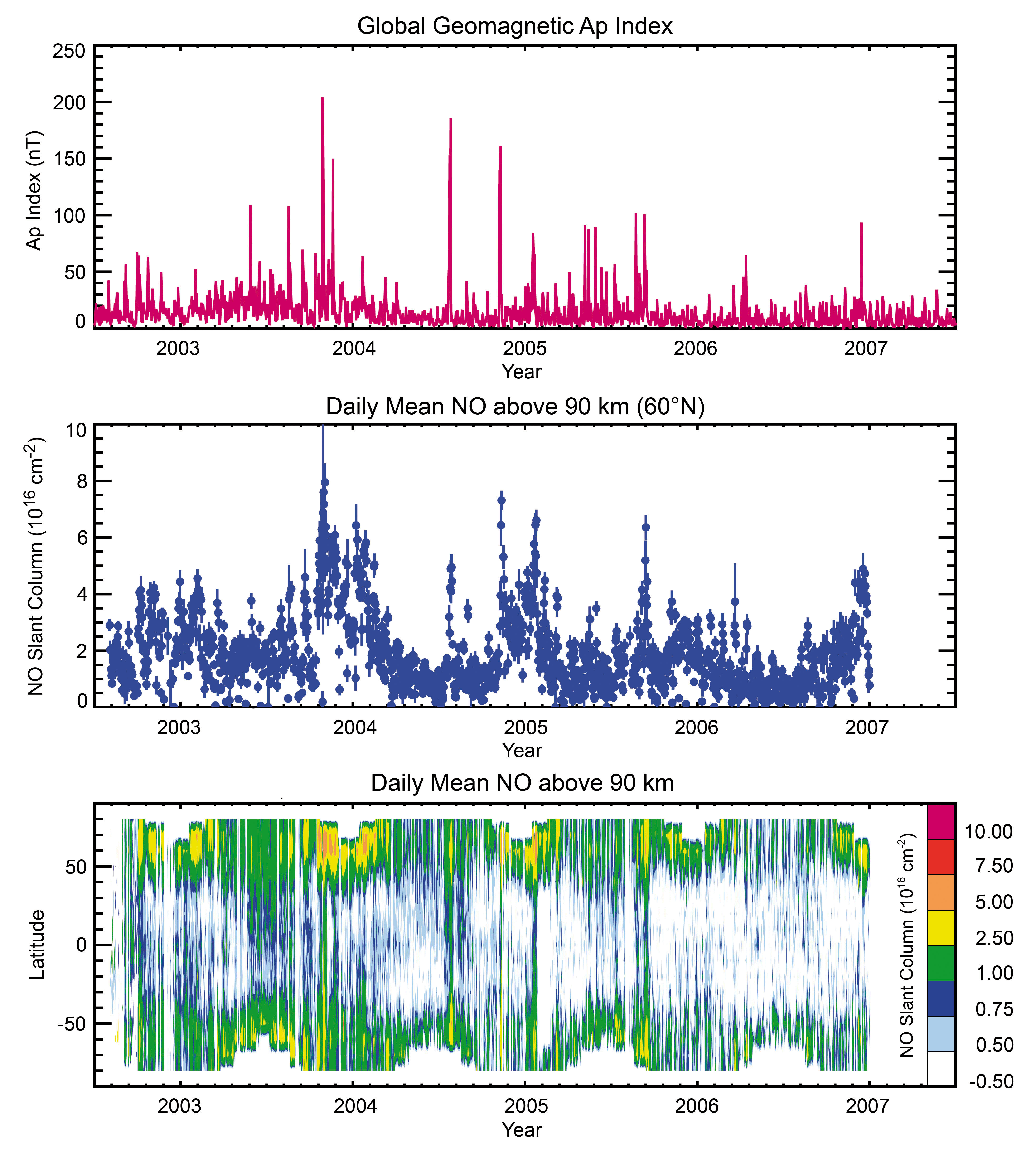
| Fig. 10-36 |
SCIAMACHY NO slant column densities, averaged daily into 10° latitude bins. Top panel: Global
Ap index, a proxy for disturbances of the geomagnetic field. Mid panel: Temporal evolution of
NO at 60°N. Lower panel: Global temporal evolution. (Courtesy: M. Sinnhuber, IUP-IFE, University of Bremen;
data courtesy Ap index: NOAA NGDC) |
|
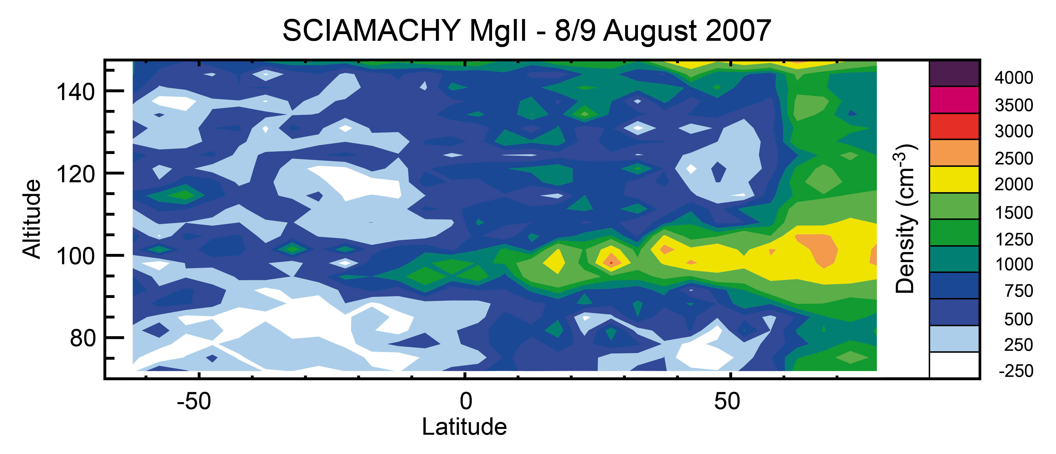
| Fig. 10-37 |
Atmospheric abundance of MgII derived from 20 orbits scanning in the mesosphere-thermosphere limb mode from 60-160 km in
August 2007. The most striking feature is the strong MgII layer around 100 km extending from high northern latitudes to the equator.
Courtesy: M. Sinnhuber, IUP-IFE, University of Bremen) |
|
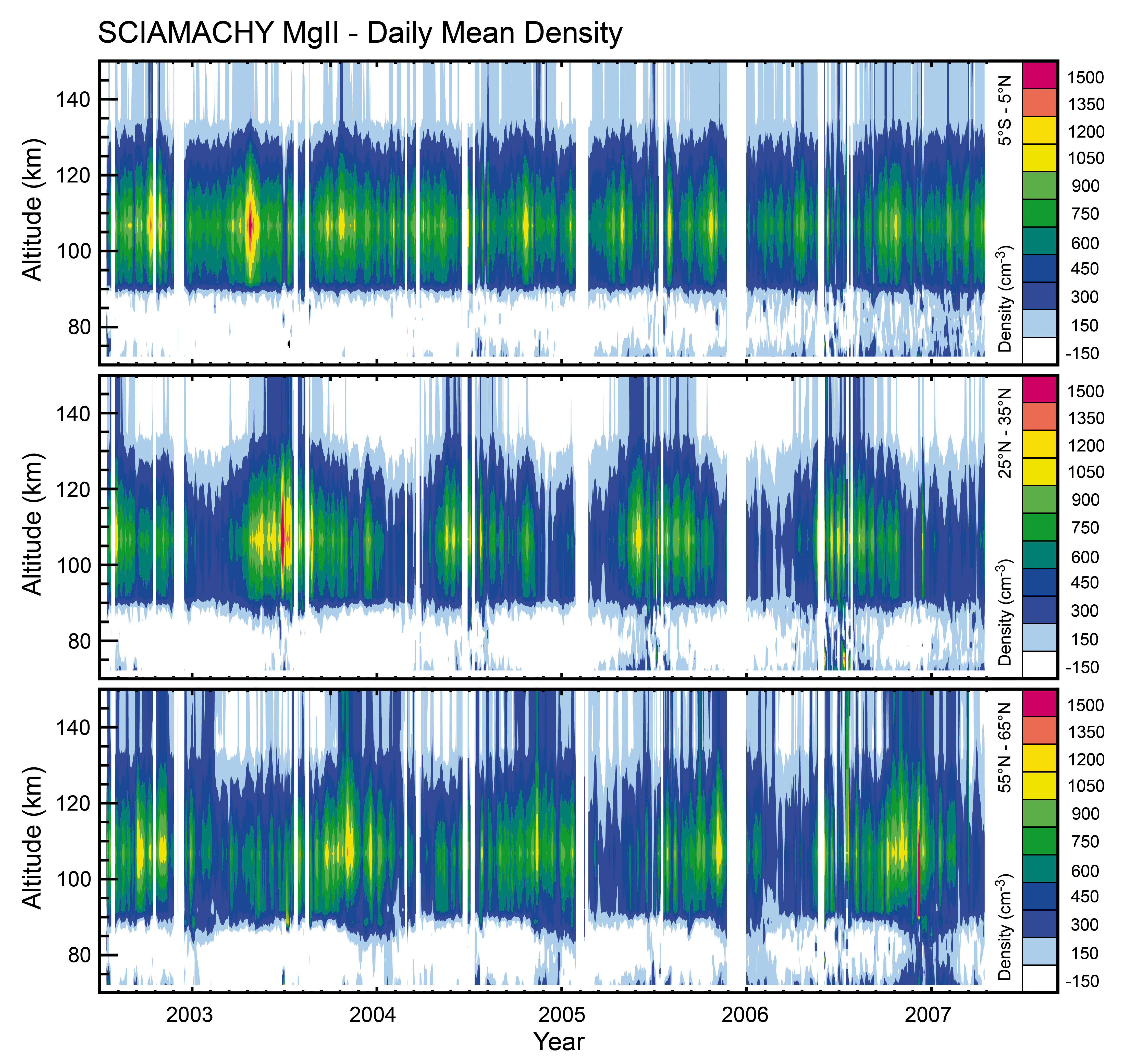
| Fig. 10-38 |
Atmospheric abundances of MgII derived from the nominal limb scanning from the surface up to 93 km.
The strong maximum around 100 km is reproduced very well, although with lower values due to the restricted vertical
resolution above 93 km. The three panels show the MgII densities at different latitude bands: 5°S-5°N (top),
25°N-35°N (mid) and 55°N-65°N (bottom). (Courtesy: M. Scharringhausen/M. Sinnhuber, IUP-IFE, University of Bremen) |
|
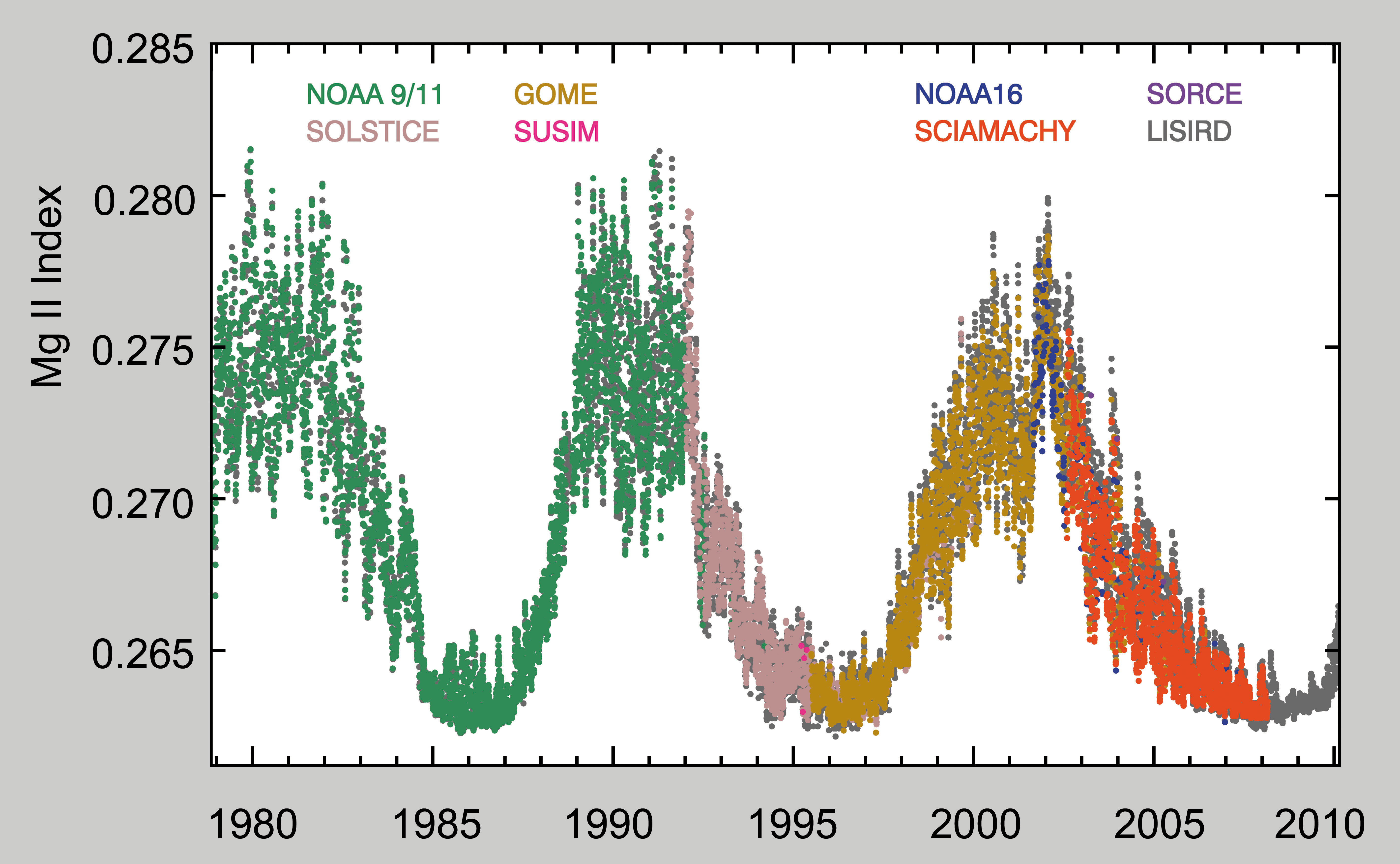
| Fig. 10-39 |
Solar activity measured via the Mg II index by several satellite instruments, including GOME and SCIAMACHY.
By combining various satellite instruments, the composite Mg II index covers more than three complete 11-year solar cycles.
(Courtesy: M. Weber, IUP-IFE, University of Bremen) |
|
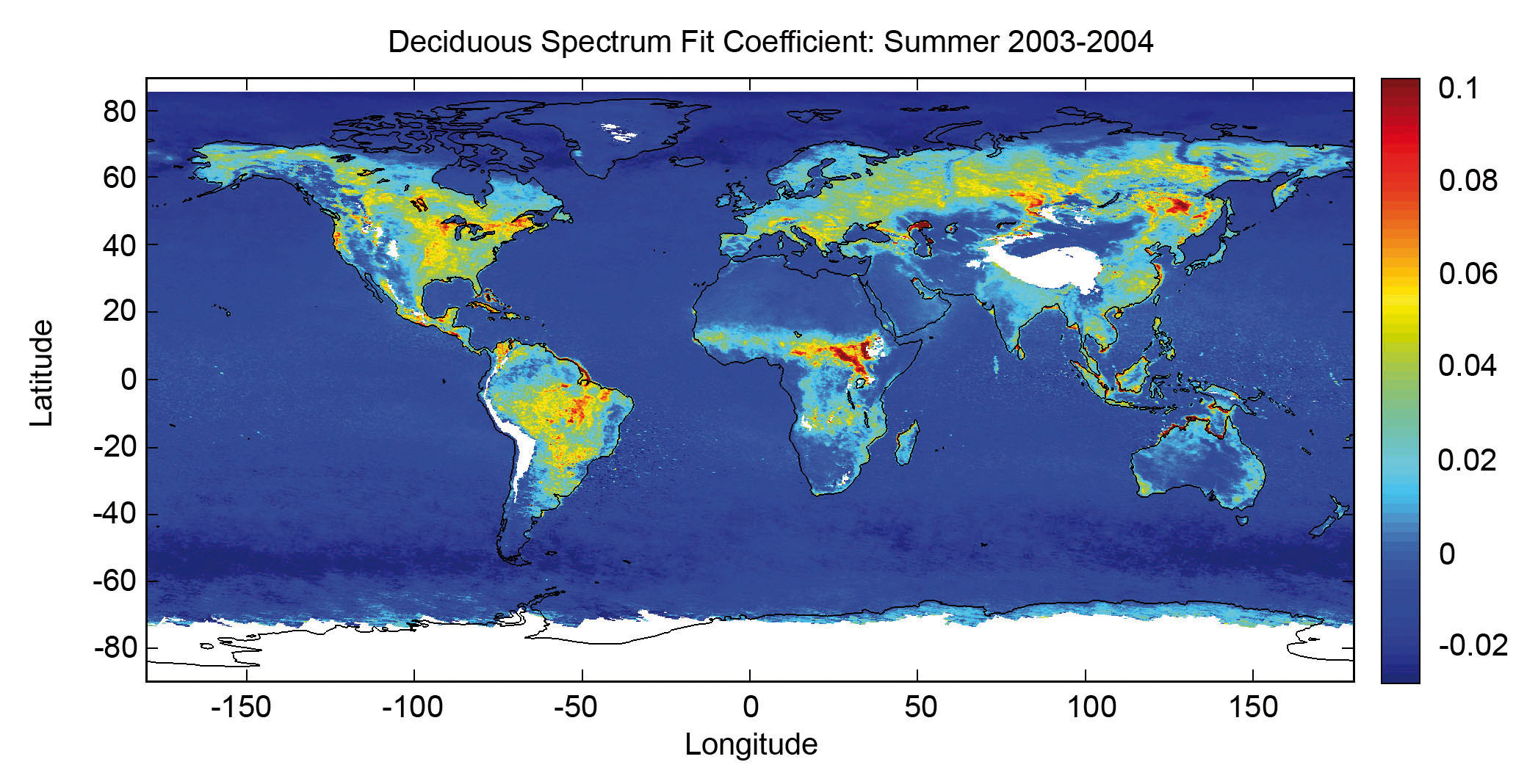
| Fig. 10-40 |
Global mean deciduous vegetation signature - DOAS fitting coefficient of the logarithm of the deciduous
vegetation spectrum - for summer 2003-2004 for cloud-free scenes. (Courtesy: T. Wagner, MPI for Chemistry, Mainz) |
|
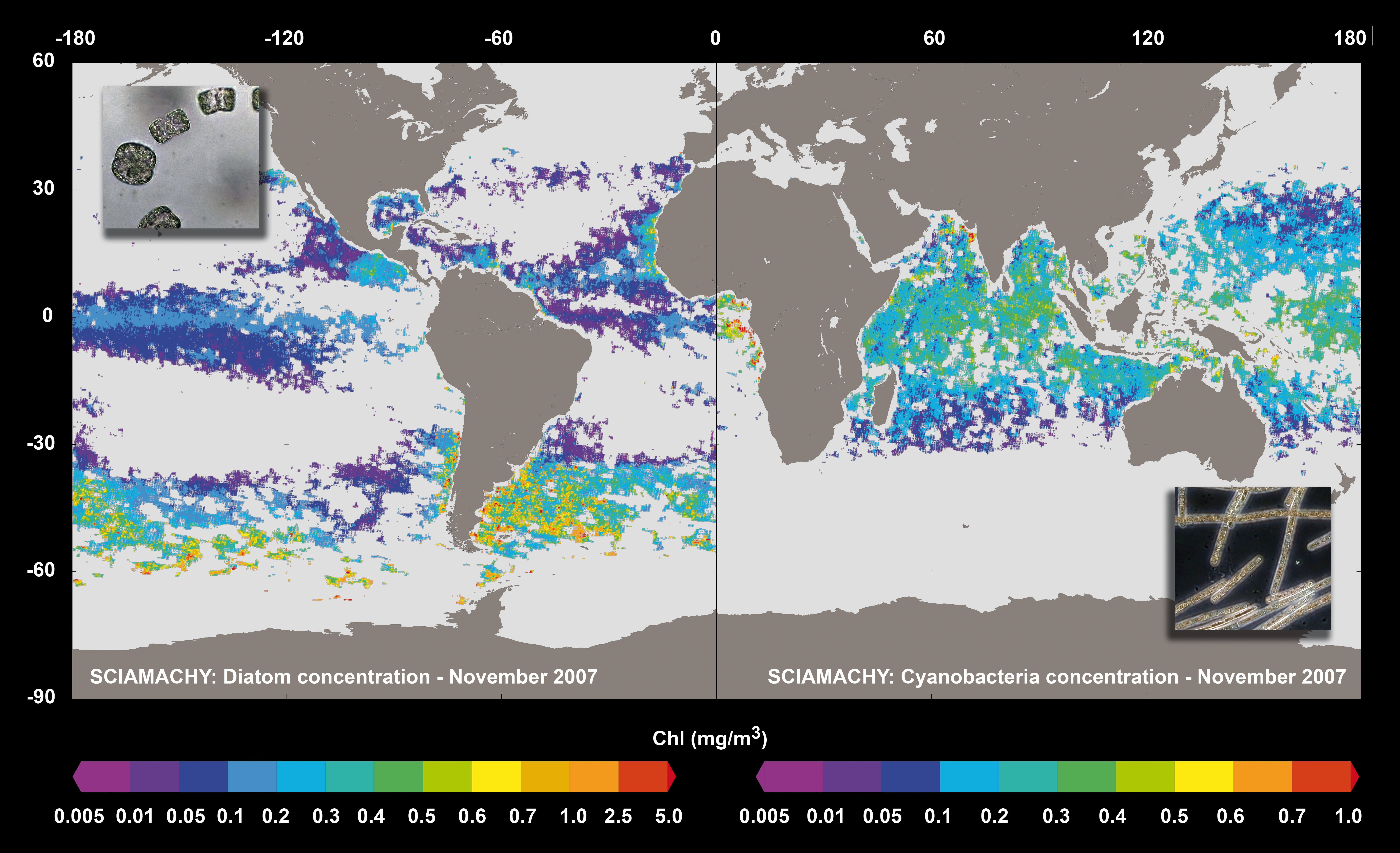
| Fig. 10-41 |
Global biomass distributions of diatoms (left hemisphere) and cyanobacteria (right hemisphere) in November 2007 as
derived from SCIAMACHY data using the PhytoDOAS method. The insets show members of the two algae groups.
(Courtesy: A. Bracher IUP-IFE, University of Bremen and Alfred Wegener Institute for Polar and Marine Research,
adapted from Bracher et al. 2009; photo diatoms: E. Allhusen, cyanobacteria: S. Kranz; both Alfred Wegener Institute
for Polar and Marine Research) |
|
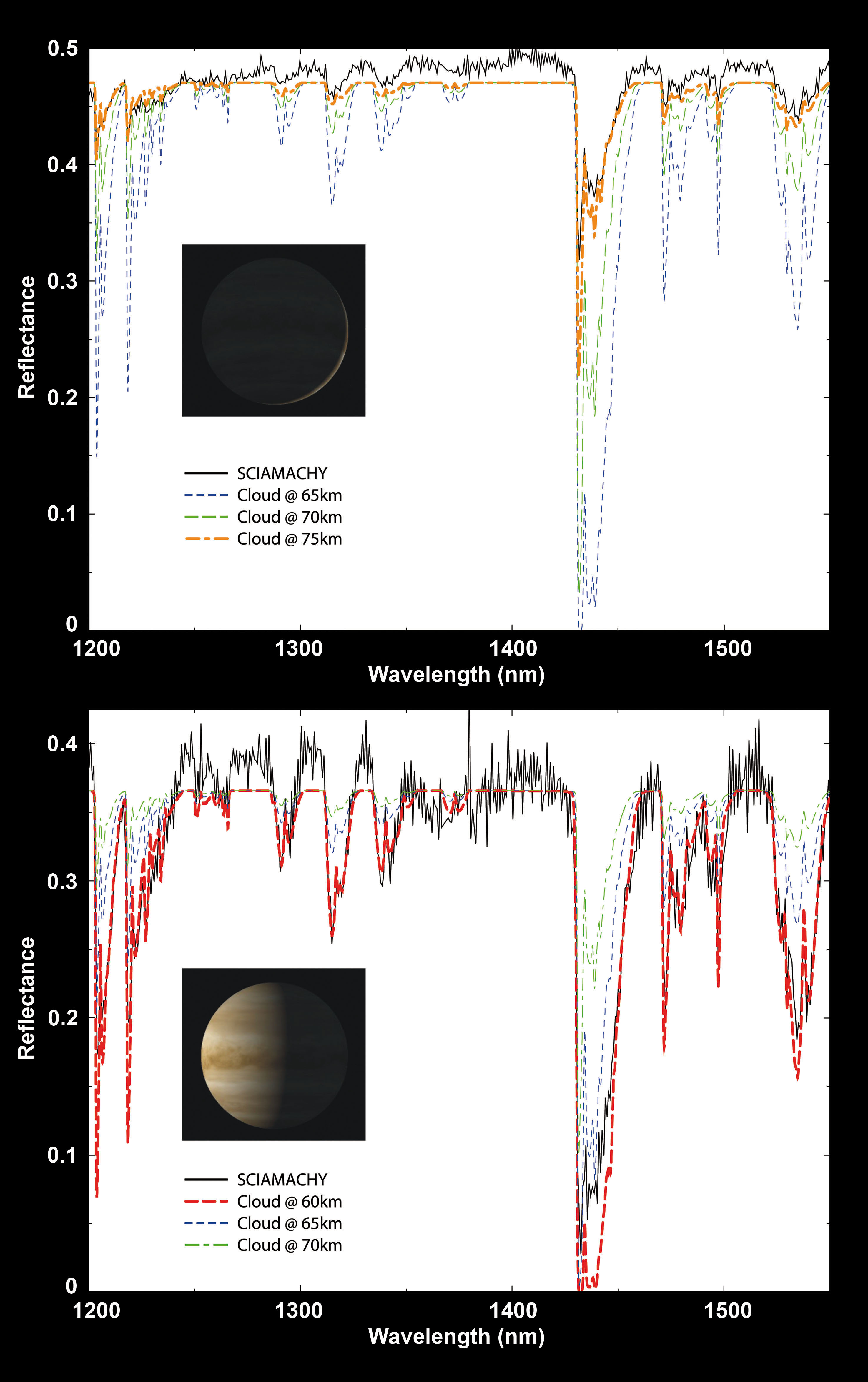
| Fig. 10-42 |
Venus reflectance from 1200 nm to 1550 nm as measured in March (top) and June (bottom) 2009. Most absorption features are due to CO2.
The spectra are modelled by using CO2 as absorber and H2SO4 clouds at different altitudes as scatterer.
The illumination conditions in the insets have been derived from the NASA/JPL Solar System Simulator.
(Courtesy: M. Vasquez, DLR-IMF) |
|
Page generated 31 August 2011